Newton's law of motion says that the force on a body is its mass times
its acceleration. Acceleration is a second derivative, so this law is a
differential equation, and it is the reason the subject exists. Newton
developed calculus in large part to study motion, and for centuries
differential equations meant, above all, the equations of mechanics: a
falling stone, a swinging pendulum, the planets going around the sun.
In this chapter we bring everything we have built to Newton's law. We
will see that for a system of many pieces it is a large nonlinear
system, so its equilibria, its linearizations, and its phase portraits
are all within reach of our tools. We will also see physics give
something back: the energy of a mechanical system never changes, and
that simple fact turns out to be a powerful method of its own, useful
far beyond physics.
13.1Newton's Law
Newton's law says that the force on a body equals its mass times its
acceleration. Suppose a system has 𝑁 pieces: masses on springs, atoms
in a molecule, planets around a sun. Write 𝑋𝑖 for the position of
piece 𝑖 and 𝑚𝑖 for its mass. The force on piece 𝑖 depends on
where all the pieces are, so
𝑚𝑖𝑋″𝑖=𝐹𝑖(𝑋1,…,𝑋𝑁),𝑖=1,…,𝑁.
Stack all the positions into one long vector 𝑋=(𝑋1,…,𝑋𝑁) and
all the forces into 𝐹=(𝐹1,…,𝐹𝑁). Then Newton's law is a single
equation,
𝑀𝑋″=𝐹(𝑋),
where 𝑀 is the diagonal matrix that multiplies each piece's
coordinates by its mass. As a first-order system, the state is the
position 𝑋 together with the velocity 𝑋′. So 𝑁 pieces moving in
the plane have a state with 4𝑁 numbers. Three stars in the plane, as
in section 11.4, already have a 12-dimensional state.
And the forces are almost never linear in 𝑋. Gravity weakens with
distance, and a spring pulls along its own direction, which changes as
it tilts. So Newton's law for a system of many pieces is a large
nonlinear system.
13.2One-Dimensional Motion
Many mechanical systems have only one way to move. A bead threaded on
a wire can only slide along the wire, a pendulum can only swing around
its circle, and a mass on a spring in a track can only slide back and
forth. The position of such a system is a single number 𝑥. But
Newton's law involves the second derivative, so the state is the
position together with the velocity 𝑣=𝑥′, and the motion is a system
in the plane. Planar systems describe exactly the motions with one way
to move. A particle moving freely in space is a different matter: it
has three coordinates of position and three of velocity, so its state
is six numbers.
Taking the mass to be 1, Newton's law is 𝑥″=𝐹, and the force can
depend on the position and on the velocity. The force of a spring
depends only on its stretch, and the force of gravity on a pendulum
depends only on its angle. These are position-dependent forces.
Drag from air or water is a velocity-dependent force: it is zero
when the particle is at rest and opposes the motion otherwise. When
both kinds are present,
𝑥″=𝑃(𝑥)+𝐷(𝑥′),
where 𝑃(𝑥) is the position-dependent force and 𝐷(𝑥′) is the drag,
with 𝐷(0)=0. As a system,
𝑥′=𝑣,𝑣′=𝑃(𝑥)+𝐷(𝑣).
To see what these systems do, let's look at a bead on a wire. Write 𝑠
for the distance along the wire from a fixed point, and ℎ(𝑠) for the
height of the wire there. Two forces act on the bead: gravity, pulling
down with strength 𝑔, and the push of the wire, which keeps the bead
on it. The wire can only push perpendicular to itself, so along the
wire, only gravity counts. The unit vector along the wire has vertical
component ℎ′(𝑠), so the component of gravity along the wire is
−𝑔ℎ′(𝑠). The acceleration along the wire is 𝑠″, so with air
resistance −𝑐𝑠′, Newton's law along the wire is
𝑠″=−𝑔ℎ′(𝑠)−𝑐𝑠′.
The position-dependent force is 𝑃(𝑠)=−𝑔ℎ′(𝑠), and the drag is
𝐷(𝑠′)=−𝑐𝑠′.
Take a W-shaped wire, with height ℎ(𝑠)=𝐴(−12𝑠2+14𝑠4),
where 𝐴>0 is small enough that the wire is never steeper than
vertical on the piece we use. Then −𝑔ℎ′(𝑠)=𝑔𝐴(𝑠−𝑠3), so
𝑠″=𝑔𝐴(𝑠−𝑠3)−𝑐𝑠′.
We are mathematicians, so we take the constant 𝑔𝐴 to be 1:
𝑠″=𝑠−𝑠3−𝑐𝑠′,
the double well from chapter 11, now with a physical meaning.
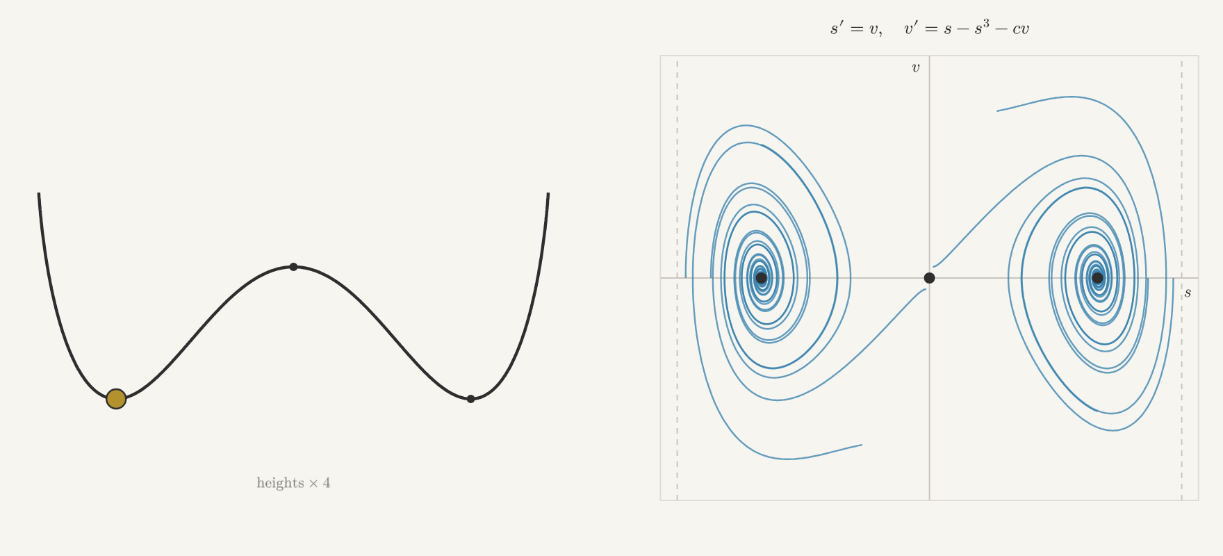
Figure 13.1 Left: a bead on a W-shaped wire, with heights drawn four times larger.
Right: trajectories of 𝑠′=𝑣, 𝑣′=𝑠−𝑠3−𝑐𝑣. Move the slider to change
the drag 𝑐, and click the right picture to release the bead.
Now the general picture. At an equilibrium, 𝑣=0 and
𝑃(𝑥0)+𝐷(0)=0. Since 𝐷(0)=0, the equilibria are the states
(𝑥0,0) with 𝑃(𝑥0)=0: drag doesn't create or remove them. For the
bead, they are the points where the wire is level, ℎ′(𝑠)=0: the top
of the middle hump, 𝑠=0, and the two bottoms, 𝑠=±1. The Jacobian
at an equilibrium is
𝐽=(01𝑃′(𝑥0)𝐷′(0)).
Its trace comes only from the drag, and its determinant, −𝑃′(𝑥0),
comes only from the position-dependent force.
If 𝑃′(𝑥0)>0, a small displacement from 𝑥0 produces a force away
from 𝑥0. The determinant is negative, so the equilibrium is a
saddle, for any drag. For the bead, 𝑃′(0)=1: a bead balanced on top
of the hump falls to one side or the other unless it starts exactly
right.
If 𝑃′(𝑥0)<0, a small displacement produces a force back toward
𝑥0, and the determinant is positive. With drag, 𝐷′(0)=−𝑐<0, so the
equilibrium is a sink. It is a spiral sink when 𝑐2<4|𝑃′(𝑥0)|. For
the bead, 𝑃′(±1)=−2, so when 𝑐2<8 the bead rocks back and forth
in the dip, less each time, and comes to rest at the bottom. With more
drag, it slides to the bottom without rocking.
A velocity-dependent force can do more than slow things down. Van der
Pol's equation from section 11.2, 𝑥″=−𝑥+(1−𝑥2)𝑥′, has a
velocity-dependent force that speeds up small motions and slows large
ones, and every motion settles onto a single attracting loop. With
velocity-dependent forces, sinks, sources, and attracting loops all
appear in one-dimensional mechanics.
Now remove the drag, so that the force depends only on position:
𝑥″=𝑃(𝑥). The trace is 0. Where 𝑃′(𝑥0)>0, the equilibrium is
still a saddle. Where 𝑃′(𝑥0)<0, it is a center. (Where 𝑃′(𝑥0)=0,
linearization fails.) There are no sinks and no sources. Set the drag
to zero in the figure: the bottoms of the wire become centers, and the
top of the hump stays a saddle.
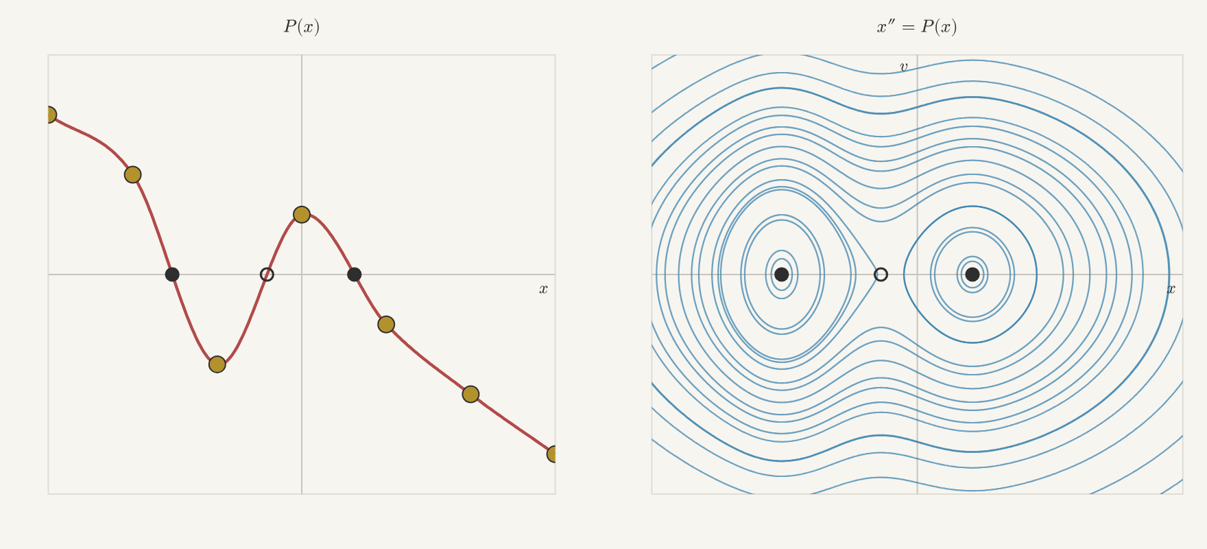
Figure 13.2 Left: the graph of a force 𝑃(𝑥); drag the points to change it.
Right: trajectories of 𝑥″=𝑃(𝑥). Each zero of 𝑃 is an equilibrium.
At a center, linearization can't decide what happens. Here a symmetry
decides it. If (𝑥(𝑡),𝑣(𝑡)) solves 𝑥′=𝑣, 𝑣′=𝑃(𝑥), then so does
(𝑥(−𝑡),−𝑣(−𝑡)): reflect a trajectory across the 𝑥-axis and reverse
its direction, and you get another trajectory. Now take an equilibrium
𝑥0 with 𝑃′(𝑥0)<0, and start a state on the 𝑥-axis just to its
right, at (𝑎,0). Near the equilibrium the flow turns like its
linearization, so the state goes around below 𝑥0 and returns to the
axis on the other side, at some (𝑏,0). Reflecting this arc gives a
trajectory from (𝑏,0) back to (𝑎,0) through the upper half-plane.
By uniqueness, that is how the state continues. So it returns to
(𝑎,0) and goes around again: the trajectory is a closed loop, and
the motion is periodic.
So when the forces depend only on position, the equilibria are saddles
and centers, and near every center the motion repeats. The same
symmetry rules out sinks entirely, even where linearization fails:
reversing time turns a sink into a source, so an equilibrium that drew
in every nearby state would also have to push them all away. Sinks need
a velocity-dependent force.
13.3Energy Conservation
In section 13.2 we learned what happens near the equilibria of
𝑥″=𝑃(𝑥): they are saddles and centers, and near a center the motion
repeats. That says nothing about states far from an equilibrium.
Release the bead from rest high on the left wall of the W. Does it stay
in the left dip, or does it cross the hump in the middle? In
section 11.1 we claimed that a state released at rest from
√2 has exactly enough energy to climb back to the top of the hump.
Now we can make that precise.
The question is about where the bead goes, not when it gets there.
So instead of looking for the solution 𝑥(𝑡), let's look for the curve
the state traces in the (𝑥,𝑣)-plane.
What do we know about that curve? At every state, the system gives us
the velocity arrow, (𝑥′,𝑣′)=(𝑣,𝑃(𝑥)), and the trajectory
through that state follows its arrow. The length of the arrow tells us
how fast the state moves along the curve: that's the when, which we
don't care about. The direction of the arrow tells us which way the
curve goes, and that direction is a slope, rise over run:
𝑣′𝑥′=𝑃(𝑥)𝑣.
So at every state with 𝑣≠0 we know the slope of the trajectory
through it. That is a slope field, just like the ones in
section 1.2, with 𝑥 in place of time and 𝑣 in place of the
unknown. The trajectories are its solution curves, so they solve
𝑑𝑣𝑑𝑥=𝑃(𝑥)𝑣.
For the bead, 𝑑𝑣𝑑𝑠=𝑠−𝑠3𝑣. We have traded a system
of two equations for a single first-order equation, and this one we can
solve, because it is separable (section 2.3). Separating
and integrating,
𝑣𝑑𝑣=𝑃(𝑥)𝑑𝑥,12𝑣2=∫𝑃(𝑥)𝑑𝑥+𝐶.
Write 𝑉(𝑥) for an antiderivative of −𝑃, so that 𝑉′=−𝑃. Then
12𝑣2+𝑉(𝑥)=𝐶. This is an implicit solution, as in
definition 2.3: each trajectory lies on a level curve of the
function
𝐸(𝑥,𝑣)=12𝑣2+𝑉(𝑥).
We needed 𝑣≠0 to find 𝐸, but we can check directly that it works
everywhere. Along any solution, by the chain rule,
𝐸′=𝑣𝑣′+𝑉′(𝑥)𝑥′=𝑣𝑃(𝑥)−𝑃(𝑥)𝑣=0.
So 𝐸 never changes. The function 𝑉 is called the potential
energy, 12𝑣2 the kinetic energy, and 𝐸 the energy.
The fact that 𝐸 is constant is conservation of energy. For the
bead, 𝑃(𝑠)=−𝑔ℎ′(𝑠), so we can take 𝑉(𝑠)=𝑔ℎ(𝑠): the potential
energy is 𝑔 times the height of the wire. With our choice 𝑔𝐴=1,
𝑉(𝑠)=−12𝑠2+14𝑠4.
Since each trajectory stays on one level curve of 𝐸, we can draw the
phase portrait without solving anything: we just draw the level curves.
Solving for 𝑣,
𝑣=±√2(𝐸−𝑉(𝑥)).
A state with energy 𝐸 can only be where 𝑉(𝑥)≤𝐸. It moves fastest
where 𝑉 is lowest, and it stops and turns around where 𝑉(𝑥)=𝐸.
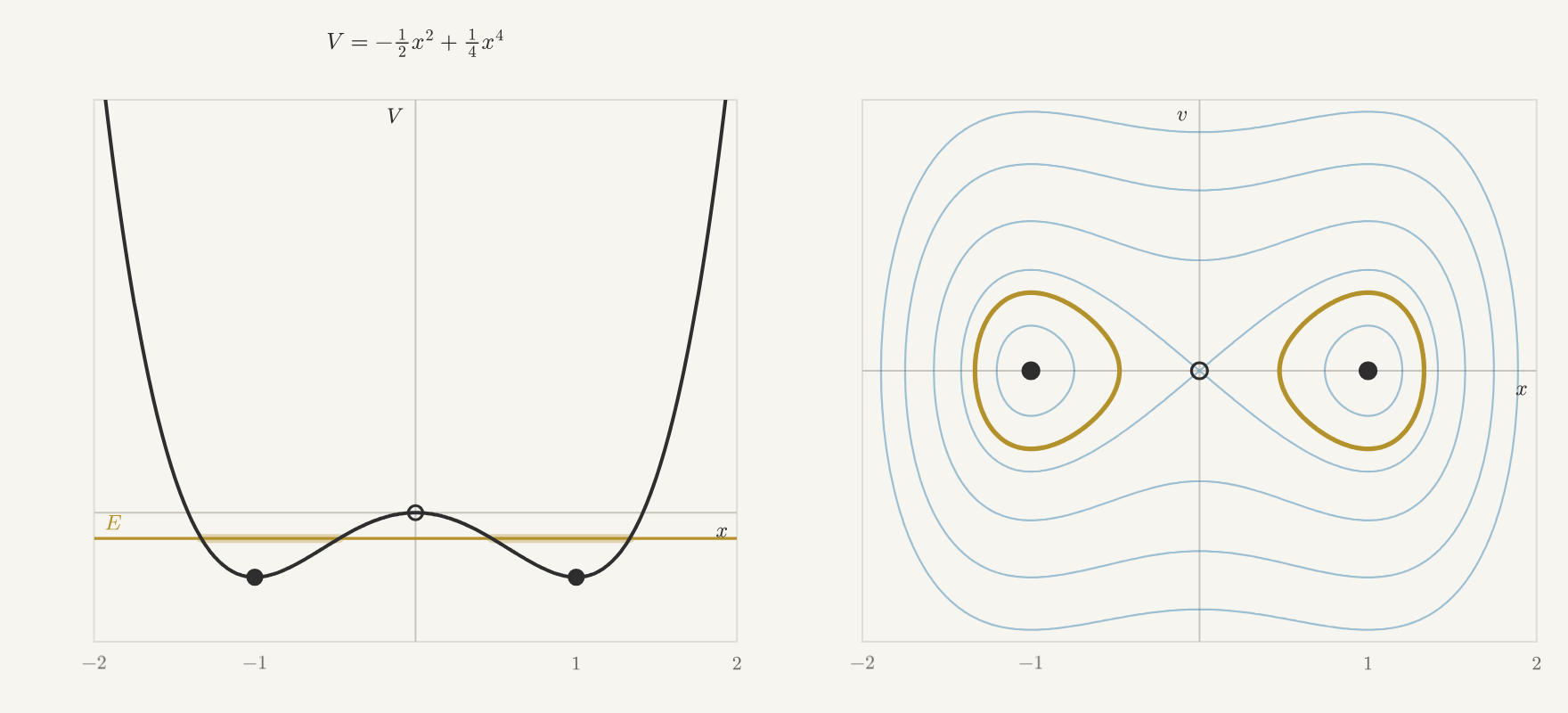
Figure 13.3 Left: the graph of the potential 𝑉, with a gold line at the energy
𝐸. Right: the level curve of 𝐸 in the (𝑥,𝑣)-plane, which is the
trajectory with that energy. Move the slider to change 𝐸, and use the
buttons to choose the force.
Now back to the bead. Released from rest at 𝑠0, it has energy
𝐸=𝑉(𝑠0). The top of the hump is at 𝑠=0, where 𝑉(0)=0. The
bottoms of the dips are at 𝑠=±1, where 𝑉=−14, and 𝑉 climbs
back to 0 at 𝑠=±√2. If |𝑠0|<√2, then 𝐸<0, and since
the bead can only be where 𝑉(𝑠)≤𝐸<0, it can never reach 𝑠=0. It
stays in its own dip. It swings between 𝑠0 and the other point on
the same side where 𝑉(𝑠)=𝑉(𝑠0), which is the point at the same
height. Released
at 𝑠0=1.3, it swings between 1.3 and about 0.56. If
|𝑠0|>√2, then 𝐸>0, and the hump is no barrier. The bead swings
across both dips, out to −𝑠0 and back. Released at exactly √2,
it has 𝐸=0 and lies on the figure-eight of section 11.1.
The equilibria are where 𝑃(𝑥0)=0, which are exactly the points where
𝑉′(𝑥0)=0. Where 𝑃′(𝑥0)<0, we have 𝑉″(𝑥0)>0, so 𝑥0 is a
local minimum of 𝑉. These are the centers of section 13.2. Where
𝑃′(𝑥0)>0, 𝑥0 is a local maximum of 𝑉, a saddle. The bead's
centers are the bottoms of the dips, and its saddle is the top of the
hump.
Energy also shows how far the repeating motion extends. Take a local
minimum 𝑥0 of 𝑉 and an energy 𝐸 a little above 𝑉(𝑥0). Near
𝑥0, the positions with 𝑉(𝑥)≤𝐸 form an interval 𝑎≤𝑥≤𝑏,
with 𝑉(𝑎)=𝑉(𝑏)=𝐸. Over that interval, the level curve of 𝐸 is a
closed loop. On its top half, 𝑣>0 and the state moves right. On its
bottom half, 𝑣<0 and it moves left. The two halves meet at the turning
points 𝑎 and 𝑏. As long as 𝑥0 is the only zero of 𝑉′ on
[𝑎,𝑏], there is no equilibrium on the loop. Then the state's speed
through the plane never drops to zero, it goes all the way around in a
finite time, and it starts over. The motion is periodic. For the bead,
this holds for every energy between −14 and 0, so every
motion that stays in one dip repeats.
For the stiffening spring 𝑥″=−𝑥−𝑥3 from section 12.4,
𝑉=12𝑥2+14𝑥4. Its only critical point is the minimum at
0, and it grows without bound in both directions. So every energy
𝐸>0 gives a closed loop: every motion of the stiffening spring is
periodic, however large.
Energy works even where linearization fails. For 𝑥″=−𝑥3, 𝑃′(0)=0,
so the Jacobian at the origin has determinant 0. In
section 13.2 we could not classify this equilibrium. But
𝑉=14𝑥4 has a minimum at 0 and no other critical point, so
again every motion is periodic.
The pendulum 𝑥″=−sin𝑥 has 𝑉=−cos𝑥. Its minima, at
𝑥=0,±2𝜋,…, are all the same hanging position. Its maxima, at
𝑥=±𝜋, are the pendulum balanced upside down, where 𝑉=1. With
energy below 1, the pendulum swings back and forth around a closed
loop. With energy above 1, 12𝑣2=𝐸−𝑉≥𝐸−1>0, so 𝑣 is never
zero, and the pendulum goes all the way over the top, again and again.
With energy exactly 1, it lies on the curves through the maxima,
which separate the two kinds of motion.
Now add drag: 𝑥″=𝑃(𝑥)+𝐷(𝑥′). Then
𝐸′=𝑣𝑣′+𝑉′(𝑥)𝑣=𝑣(𝑃(𝑥)+𝐷(𝑣))−𝑃(𝑥)𝑣=𝑣𝐷(𝑣).
Drag opposes the motion, so 𝐷(𝑣) has the opposite sign to 𝑣, and
𝑣𝐷(𝑣)<0 whenever 𝑣≠0. Energy decreases whenever the state is
moving. For the bead, 𝐸′=−𝑐𝑣2. (We have seen this before. For the
springs 𝑥″=−𝑥∓(𝑥′)3 in section 12.4, the quantity
𝑥2+𝑣2 we followed is 2𝐸, and (𝑥2+𝑣2)′=∓2𝑣4 is this formula
with 𝐷(𝑣)=∓𝑣3.)
Once the bead's energy drops below 0, the potential energy at the top
of the hump, the bead can never reach 𝑠=0 again. It is trapped in whichever
dip it is in at that moment. This is why the basins in
figure 11.3 come in bands. A bead released far out
starts with a lot of energy, and it crosses the hump again and again,
losing energy as it goes. The dip it ends in is the one it is in when
its energy drops below 0.
The same computation works for many pieces. Suppose there is one
function 𝑉(𝑋) of all the positions such that the force on each piece
is 𝐹𝑖=−∇𝑖𝑉, where ∇𝑖𝑉 is the gradient of 𝑉 with
respect to 𝑋𝑖. Then the energy
𝐸=12∑𝑖𝑚𝑖|𝑋′𝑖|2+𝑉(𝑋)
is constant:
𝐸′=∑𝑖𝑚𝑖𝑋′𝑖⋅𝑋″𝑖+∑𝑖∇𝑖𝑉⋅𝑋′𝑖=∑𝑖𝑋′𝑖⋅(𝐹𝑖−𝐹𝑖)=0.
A spring of stiffness 𝑘 and natural length 𝐿0 joining pieces 𝑖
and 𝑗 has 𝑉=12𝑘(|𝑋𝑖−𝑋𝑗|−𝐿0)2. Constant gravity
pulling down on piece 𝑖 has potential 𝑚𝑖𝑔𝑦𝑖, where 𝑦𝑖 is
its height, just as for the bead. When several forces act, we add their
potentials. With one way to move, a level set of 𝐸 is a curve, so the
energy determines each trajectory. With more pieces, a level set is
much bigger. For a single particle moving freely in space, the state
has six numbers, and a level set of 𝐸 is five-dimensional. Then 𝐸
no longer tells us the trajectory, but it still tells us where the
state can go: it stays where 𝑉(𝑋)≤𝐸.
Conserved quantities are useful far outside physics. In
section 11.2 we followed the hare–lynx model 𝐻′=𝐻(1−𝐿),
𝐿′=𝐿(𝐻−1) around what looked like closed loops, while still trusting
the computation that the loops close. There are no masses or forces
here, but there is a conserved quantity:
𝐺=𝐻−ln𝐻+𝐿−ln𝐿.
You can find 𝐺 the same way we found 𝐸, by separating the equation
for 𝑑𝐿/𝑑𝐻; see the problems at the end of this chapter. Along a
solution,
𝐺′=(1−1𝐻)𝐻′+(1−1𝐿)𝐿′=(𝐻−1)(1−𝐿)+(𝐿−1)(𝐻−1)=0.
So each trajectory stays on one level curve of 𝐺. The function
𝑢−ln𝑢 decreases until 𝑢=1, increases after, and grows without
bound as 𝑢→0 and as 𝑢→∞. So 𝐺 is smallest at the
equilibrium (1,1), and its level curves are closed loops around it.
The only equilibrium in the quadrant is (1,1), which is not on any of
these loops. So the populations go all the way around and return to
where they started: the loops really close.
13.4Linearization Around an Equilibrium
Suppose the system can rest at 𝑋0, so 𝐹(𝑋0)=0. To see what
happens nearby, we linearize, just as in chapter 12. Write
𝑋=𝑋0+𝑈. Since 𝑋0 is constant, 𝑋″=𝑈″, and the tangent
approximation from section 12.3 gives
𝐹(𝑋0+𝑈)≈𝐹(𝑋0)+𝐷𝐹(𝑋0)𝑈=𝐷𝐹(𝑋0)𝑈, where 𝐷𝐹(𝑋0) is the
Jacobian of 𝐹 at 𝑋0. When the forces come from a potential,
𝐹=−∇𝑉, this Jacobian is minus the matrix 𝐾 of second
derivatives of 𝑉 at 𝑋0. So near rest,
𝑀𝑈″≈−𝐾𝑈.
This is exactly the equation of chapter 10. Every mechanical system near
a resting state, whatever its forces, vibrates in modes. That is why we
found modes in springs, buildings, and molecules: each was the
linearization of a nonlinear system near rest. Recall the row of
stretched springs from section 10.1. If each spring obeys
Hooke's law, with stiffness 𝑘 and natural length 𝐿0, the exact
sideways pull of a spring whose ends differ in height by 𝛿 is
𝑘(1−𝐿0/√𝑎2+𝛿2)𝛿. Its linearization at
𝛿=0 is 𝑘(1−𝐿0/𝑎)𝛿=𝑇0𝛿/𝑎, since the spring's
tension is 𝑇0=𝑘(𝑎−𝐿0). That is exactly the force we used there.
With one piece on a line, 𝐾 is the number 𝑉″(𝑥0), and the
linearization is 𝑢″=−𝑉″(𝑥0)𝑢. At a valley, this is a spring with
frequency √𝑉″(𝑥0). For the pendulum, 𝑉″(0)=cos0=1, so
small swings follow 𝑢″=−𝑢, with period 2𝜋. For the double well,
𝑉″(±1)=2, so small oscillations in either well have frequency
√2. At a hilltop, 𝑉″(𝑥0)<0, and the linearization is a saddle.
Will the system actually stay near a resting state? Linearization can't
tell us. At a valley of 𝑉, where all the eigenvalues of 𝐾 are
positive, every mode oscillates, so the linearization rotates in each
mode's plane. These are centers, exactly the case where linearization
can't decide. But energy can. Suppose 𝑋0 is the bottom of a valley,
and measure 𝑉 so that 𝑉(𝑋0)=0. A state that starts near 𝑋0 with
a small velocity has a small energy 𝐸. Since 𝐸 never changes and
kinetic energy is never negative, 𝑉(𝑋)≤𝐸 for all time, and the
kinetic energy is at most 𝐸. So the state stays in the small region
around 𝑋0 where 𝑉≤𝐸, moving slowly, forever. Near the bottom of
a valley, the system stays near rest.
13.4.1The Elastic Pendulum
Here is a system where the nonlinear terms do something the modes never
could. Hang a mass from a spring that can both stretch and swing, like a
pendulum whose rod is a spring. With the pivot at the origin, mass 1,
stiffness 𝑘, natural length 𝐿0, and gravity 𝑔 pulling down,
Newton's law is
𝑋″=−𝑘(|𝑋|−𝐿0)𝑋|𝑋|−𝑔(01).
The first term is the spring's pull, along the spring, proportional to
its stretch. At rest the mass hangs straight down, where the spring's
pull balances gravity: 𝑋0=(0,−ℓ) with ℓ=𝐿0+𝑔/𝑘. Near rest,
the linearization has two modes: bouncing up and down with frequency
√𝑘, and swinging side to side with frequency √𝑔/ℓ,
like a pendulum of length ℓ.
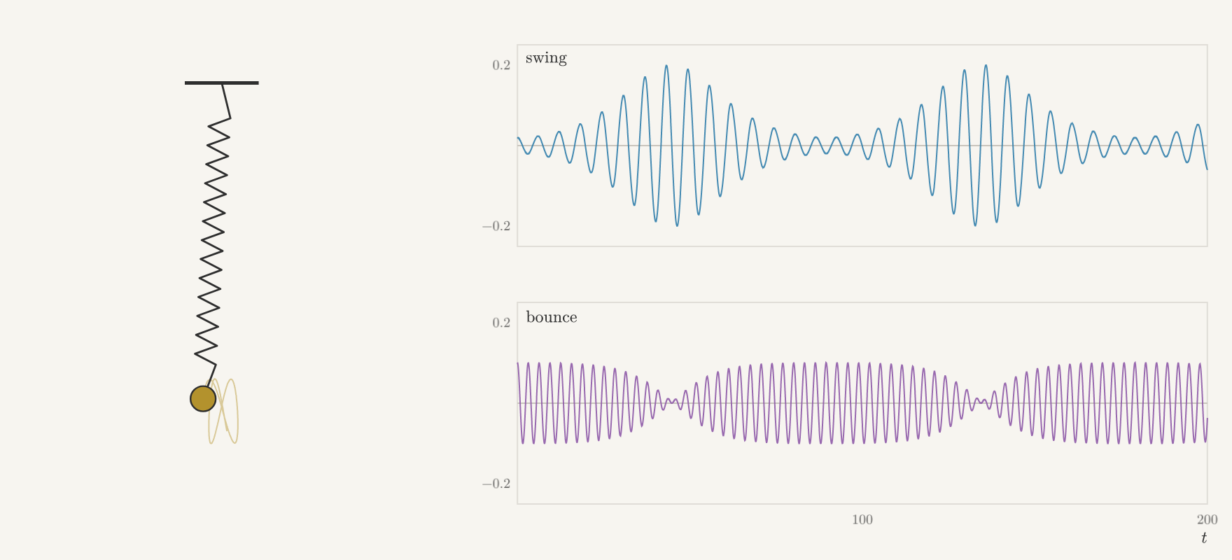
Figure 13.4 A mass on a spring that can bounce and swing, with plots of the size of
its swing and of its bounce over time. The buttons choose the
stiffness: tuned so that the bounce is twice as fast as the swing, or
not.
In the linearization, each mode keeps its own energy forever. If you
start the mass bouncing with only a tiny swing, the swing stays tiny.
The real spring usually behaves the same way. But tune it so that the
bounce is exactly twice as fast as the swing, with 𝑘=4𝑔/ℓ, and
something new happens: the bounce slowly dies down while the swing
grows, then the swing dies down while the bounce grows, back and forth.
The energy moves between the modes, and only the nonlinear terms can
move it.