In chapter 12 we learned to read the flow near an equilibrium from
its linearization. Every system there had fixed numbers in it. But models
come with parameters: a harvesting rate, a drag, a growth rate. In
section 11.3 we saw that moving a parameter can change what a
system does completely. There, we could only watch it happen in pictures.
In this chapter we study how and where it happens: how equilibria appear,
disappear, and change type as a parameter moves, and why linearization
fails at exactly those parameter values.
14.1Bifurcation Diagrams
In section 4.2.2 we harvested fish from a pond at a constant rate of 𝐻
fish per year:
𝑃′=𝑃(1−𝑃200)−𝐻.
For 𝐻=32, the population had a threshold at 40 and a stable
equilibrium at 160. As we raised 𝐻, the two moved toward each other.
At 𝐻=50 they met at 100, and for any larger harvest there were no
equilibria at all.
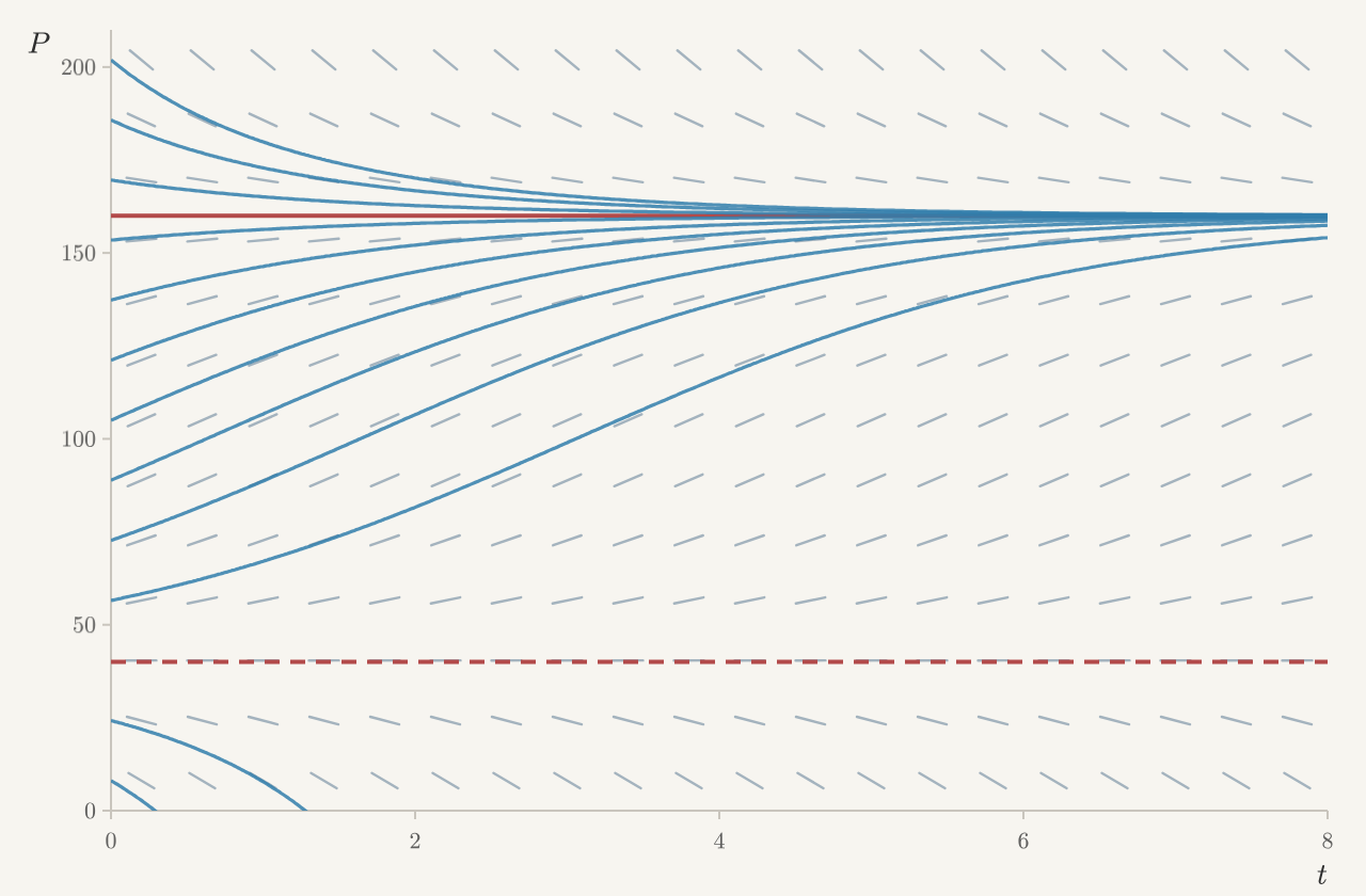
Each value of 𝐻 gives a different equation. Let's look at its
solutions.
Figure 14.1 The slope field and solutions of 𝑃′=𝑃(1−𝑃/200)−𝐻, with the equilibria
as red lines: solid where nearby solutions approach, dashed where they
move away. Move the slider to choose the harvest 𝐻.
For a harvest below 50, solutions that start above the lower
equilibrium level off at the upper one, and solutions that start below it
fall to zero. Raise the harvest past 50 and the red lines are gone:
every solution falls.
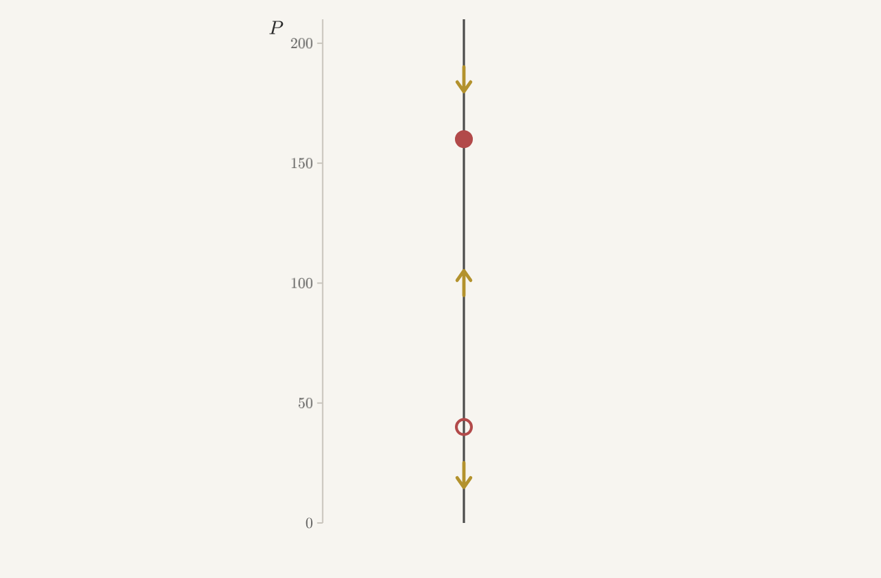
For the long run, this picture holds more than we need. All that matters
is where the equilibria are and which way solutions move between them. So
we can collapse the picture onto a single vertical line: mark the
equilibria, and draw arrows toward or away from them, pointing up where
𝑃′>0 and down where 𝑃′<0. This is the phase line of
section 3.5.
Figure 14.2 The phase line of 𝑃′=𝑃(1−𝑃/200)−𝐻: the equilibria, filled where they
attract and open where they repel, with arrows showing which way the
population moves. Move the slider to choose the harvest 𝐻.
As the harvest grows, the two equilibria on the phase line move toward
each other, meet at 𝐻=50, and disappear. Instead of watching one phase
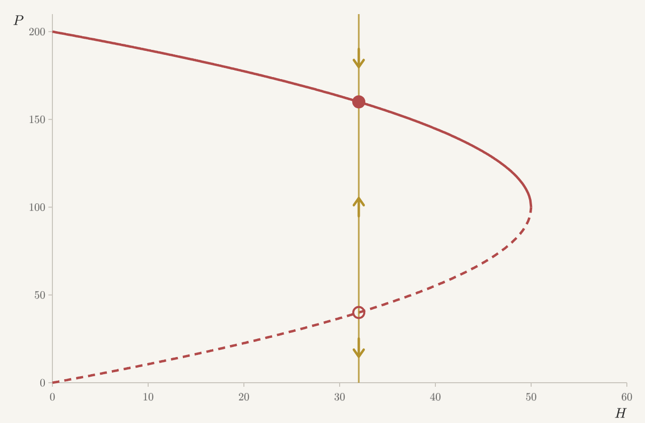
line change, we can stand the phase lines for every harvest side by side.
Figure 14.3 The equilibria of 𝑃′=𝑃(1−𝑃/200)−𝐻 for every harvest 𝐻, solid red
where they attract and dashed where they repel. The gold line is the
phase line for the harvest chosen with the slider.
To draw the curve, we solve 𝑃−𝑃2/200=𝐻 for 𝑃. Multiplying by 200
and rearranging gives 𝑃2−200𝑃+200𝐻=0, so
𝑃=100±√10000−200𝐻.
For 𝐻<50 there are two equilibria, the upper one stable and the lower
one a threshold. At 𝐻=50 the square root is zero and they meet. For
𝐻>50 there are none. A picture like this, showing the equilibria and
their stability for every value of a parameter, is called a bifurcation
diagram. A parameter value where the phase portrait changes in a basic
way, like 𝐻=50 here, is called a bifurcation. This kind, where a
stable equilibrium and an unstable one move together, collide, and
disappear, is a saddle-node bifurcation. The name comes from its
version in the plane, where the two equilibria that collide are a saddle
and a sink or source.
Linearization tells us which branch is which. For a single equation
𝑃′=𝑓(𝑃), the Jacobian is just the derivative 𝑓′. So near an
equilibrium 𝑃∗, writing 𝑃=𝑃∗+𝑢, the linearization is
𝑢′=𝑓′(𝑃∗)𝑢.
The equilibrium attracts when 𝑓′(𝑃∗)<0 and repels when 𝑓′(𝑃∗)>0.
Here 𝑓(𝑃)=𝑃−𝑃2/200−𝐻, so 𝑓′(𝑃)=1−𝑃/100. This is negative above
𝑃=100 and positive below it. So the upper branch attracts and the lower
branch repels, just as the phase lines show.
At the bifurcation itself, 𝑃=100, and 𝑓′(100)=0: the linearization
fails exactly there. That is no coincidence. Picture the graph of 𝑓, the
parabola from section 4.2.2 shifted down by 𝐻. An equilibrium is a
place where the graph crosses zero. If it crosses with nonzero slope, then
moving the graph up or down a little still leaves a crossing nearby, so
the equilibrium survives a small change in 𝐻. An equilibrium can only
appear or disappear where the graph touches zero without crossing, that
is, where
𝑓(𝑃)=0and𝑓′(𝑃)=0.
Solving these together finds the bifurcation. Here 𝑓′(𝑃)=0 gives
𝑃=100, and then 𝑓(100)=0 gives 𝐻=50.
So the largest harvest the pond can sustain, which we found in
section 4.2.2, is a bifurcation value. For any harvest above 50 fish
per year, the pond has no equilibrium at all, and every population
eventually collapses.
14.2Transcritical and Pitchfork Bifurcations
Equilibria don't always appear and disappear. Sometimes they stay, but
trade stability.
In section 4.2.2 we noted that a constant quota keeps removing fish from
an empty pond. Suppose instead that we remove a fixed fraction 𝑞 of the
fish each year:
𝑃′=𝑃(1−𝑃200)−𝑞𝑃=𝑃(1−𝑞−𝑃200).
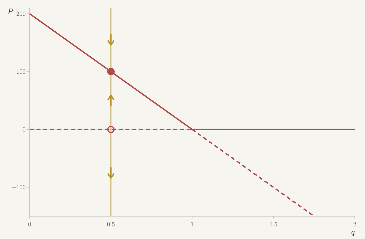
Now there are always two equilibria: the empty pond 𝑃=0, and
𝑃=200(1−𝑞).
Figure 14.4 Equilibria of 𝑃′=𝑃(1−𝑞−𝑃/200) for each fishing fraction 𝑞, solid red
where they attract and dashed where they repel. Move the slider to choose
𝑞; the gold line is the phase line for that 𝑞.
As 𝑞 rises toward 1, the second equilibrium slides down to 0. Past
𝑞=1 it is negative, which has no meaning for a pond, but the mathematics
continues. Linearization shows what changes. Here
𝑓(𝑃)=𝑃(1−𝑞)−𝑃2/200, so 𝑓′(𝑃)=1−𝑞−𝑃/100. At the empty pond,
𝑓′(0)=1−𝑞. At the other equilibrium, 𝑓′(200(1−𝑞))=−(1−𝑞). For
𝑞<1, the fish population attracts and the empty pond repels. For 𝑞>1,
they swap. At 𝑞=1 the two equilibria meet, both derivatives are zero,
and the linearization fails again. This is a transcritical
bifurcation: two equilibria pass through each other and exchange
stability.
The two harvesting policies end very differently. With proportional
harvesting, the population shrinks steadily as 𝑞 grows, reaching zero
only at 𝑞=1. With a constant quota, the stable population is still 100
at 𝐻=50, and then any larger quota sends it to collapse.
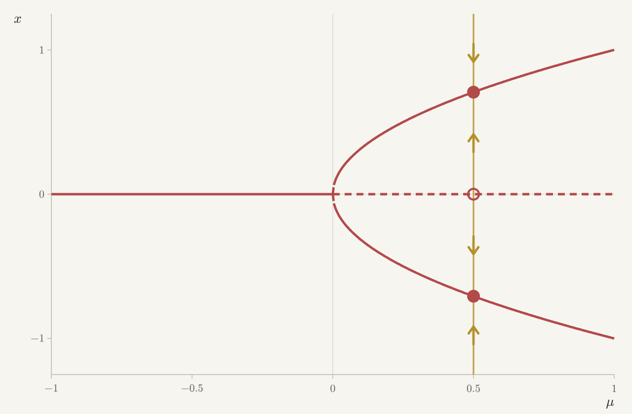
Finally, an equilibrium can split into three. Consider
𝑥′=𝜇𝑥−𝑥3,
where 𝜇 is a parameter. The origin is always an equilibrium. When
𝜇>0 there are two more, 𝑥=±√𝜇.
Figure 14.5 Equilibria of 𝑥′=𝜇𝑥−𝑥3 for each 𝜇, solid red where they attract
and dashed where they repel. Move the slider to choose 𝜇; the gold
line is the phase line for that 𝜇.
Here 𝑓′(𝑥)=𝜇−3𝑥2. At the origin, 𝑓′(0)=𝜇, so the origin attracts
when 𝜇<0 and repels when 𝜇>0. At 𝑥=±√𝜇,
𝑓′=𝜇−3𝜇=−2𝜇<0, so both new equilibria attract. As 𝜇 increases
through 0, the stable origin becomes unstable and hands its stability to
a pair of new equilibria, one on each side. Once more, the linearization
fails at the bifurcation: at 𝜇=0, 𝑓′(0)=0. The diagram looks like a
pitchfork, and this is called a pitchfork bifurcation.
The pair appears together because of a symmetry. Replacing 𝑥 by −𝑥
turns the equation into itself, since 𝑓(−𝑥)=−𝑓(𝑥). So whenever 𝑥 is
an equilibrium, so is −𝑥. A ruler squeezed from both ends behaves this
way: past a certain force, it buckles to the left or to the right, and by
symmetry neither side is preferred.