Chapter 2

Finding Solutions

In the last chapter we learned what a differential equation says. A local rule assigns a slope at each possible time and state, and an initial condition specifies a point our solution must pass through. Drawing the slope field lets us begin to picture the possible histories. But how do we actually find one? How do we turn the local rule into a function we can evaluate, or a calculation we can carry out?

In one sense, that question is the subject of this entire book! But our first attempt will be deliberately modest. We will focus mostly on one unknown function and one first-order equation

𝑦' = 𝐹 (𝑡, 𝑦) .

We will take advantage of this simple situation to explore the different things one might want when asking for a solution---there's no one-size-fits-all technique, nor should there be! Sometimes we want a formula for an answer, something we can recognize from calculus or derive using its techniques, then plug things into and get precise predictions. Other times we may know that whatever formula exists is too complicated to be useful, or that it's essentially impossible to write down---in these cases we might prefer a numerical solution: an algorithm that follows the local rule to give us good approximations to the answer quickly, while avoiding thousands of pages of calculus and algebra. And other times we may find a simple plot reveals enough information that we don't need a formula or rigorous numerics at all.

We will spend a little more time on the 'formula' case here, but not because it is necessarily more important. This chapter is also a chance to put some familiar calculus back to work: antidifferentiation, the chain rule, and the product rule. The point will not be to memorize a new collection of formulas. It will be to look at an equation and ask: is there a piece of calculus here which we already know how to undo?

2.1Guessing and Checking Solutions

First things first: how do we confirm that we have a solution to a differential equation? If we are given a formula, we differentiate it and substitute into the equation to check that the two sides agree. If there is an initial condition, we check that too. We know how to differentiate elementary functions, so when someone proposes an elementary formula as a solution, we have a direct way to check their answer ourselves!

This opens up a possibility: guess and check could be a rigorous solution technique. We might recognize a function whose derivatives behave the way the equation asks, or try a few possibilities until something works. However we arrive at our guess, once we verify that it satisfies the equation and the initial condition, we have found a solution.

The simplest version of this idea is

𝑦' = 𝑦 .

We need a function which is equal to its own derivative, so $𝑒 𝑡$ is a natural guess. Multiplying by any constant still works:

𝑑 𝑑 𝑡 (𝐶 𝑒 𝑡) = 𝐶 𝑒 𝑡 .

Thus $𝑦 = 𝐶 𝑒 𝑡$ gives an entire family of solutions. One initial condition selects the value of $𝐶$ , and therefore selects one member of this family.

Figure 2.1 The family $𝑦 = 𝐶 𝑒 𝑡$ threading the slope field of $𝑦' = 𝑦$ . Every member satisfies the equation; the constant $𝐶$ is chosen by one piece of data. The $𝐶 = 0$ member lies exactly on the $𝑡$ -axis: the axis itself is a solution. In the live figure, drag the gold point — the readout answers with the formula.

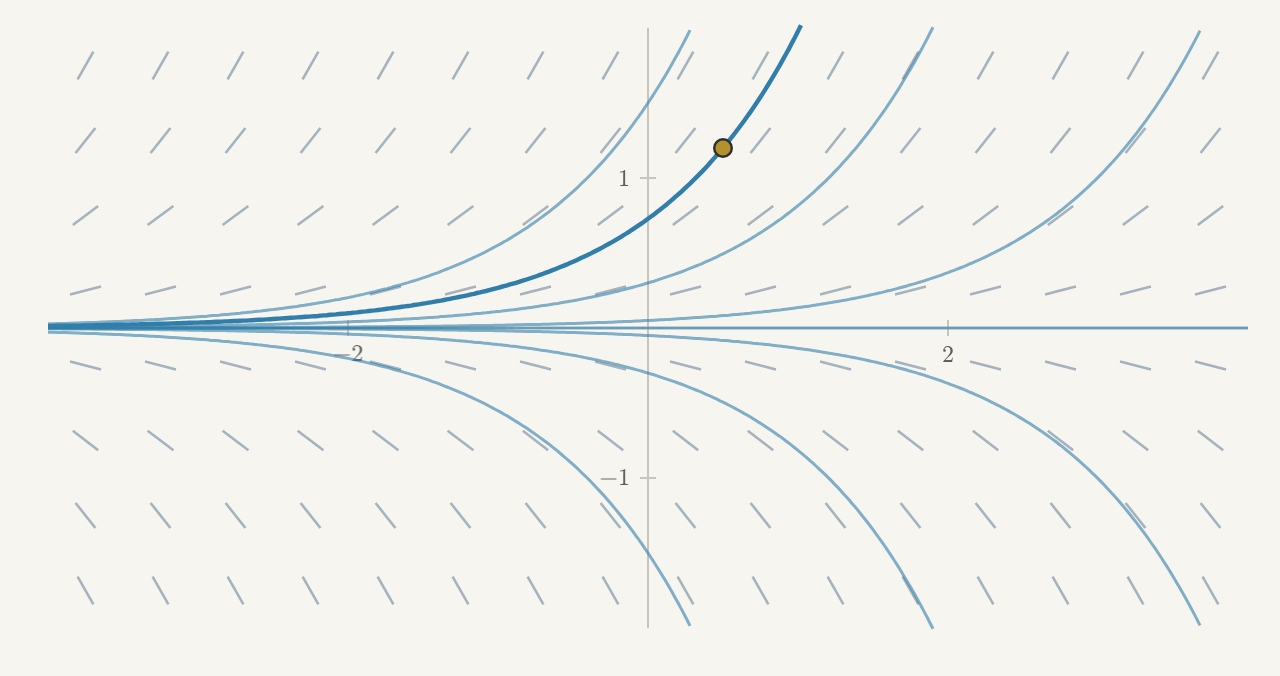
Recall the differential equation we placed beside its algebraic counterpart at the very beginning of the book:

𝑓 ″ + 4 𝑓' = 5 𝑓 .

At first this looks intimidating, since it asks for a sum of derivatives of $𝑓$ to somehow equal a multiple of $𝑓$ . But one (simple!) way this could happen is if each derivative were itself a multiple of $𝑓$ . Then we would just be adding multiples of the same function, and it would be no surprise to get another multiple of it. And we actually know functions whose derivatives are multiples of themselves---exponentials!

This suggests we might guess $𝑒 𝑟 𝑡$ as a solution. Then $𝑓' = 𝑟 𝑒 𝑟 𝑡$ and $𝑓 ″ = 𝑟 2 𝑒 𝑟 𝑡$ , so substitution gives

(𝑟 2 + 4 𝑟) 𝑒 𝑟 𝑡 = 5 𝑒 𝑟 𝑡 .

Cancelling the exponential from both sides (since it is never zero, we can do this) reduces the differential equation to the algebraic equation

𝑟 2 + 4 𝑟 = 5 .

Its solutions are $𝑟 = 1$ and $𝑟 = - 5$ , giving the two functions $𝑒 𝑡$ and $𝑒 - 5 𝑡$ . The resemblance between the two opening equations was not only superficial: the exponential guess turns the differential equation back into the algebraic one.

Remembering other relationships from calculus can extend our ability to guess (and check) even more equations. For the normalized spring equation

𝑥 ″ = - 𝑥,

the functions $c o s 𝑡$ and $s i n 𝑡$ are natural candidates, since taking two derivatives negates each of them. And a direct check shows that these work---as does any sum or multiple of them, in fact! The spring oscillates just as we would expect.

Guessing and checking is a genuine solution technique, but not a systematic one: it works when we can recognize the right kind of function. So what else can we borrow from calculus? Not only remembered relationships, but the techniques themselves.

2.2Antidifferentiation

So far we have borrowed facts from calculus to help us guess. But we can also borrow the techniques of calculus to produce solutions more systematically. In the easiest case, the differential equation simply tells us the derivative of the function we are looking for:

𝑦' = 𝑔 (𝑡),

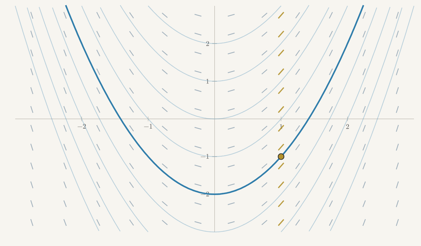
and the important thing here is that the right-hand side depends only on $𝑡$ , not on $𝑦$ . The slope does not care about the current value of the function at all; it cares only about the input. At a fixed time $𝑡$ , every point $(𝑡, 𝑦)$ therefore receives exactly the same slope, no matter how high or low the point lies. In the slope field, this shows up as entire vertical columns of identical ticks.

Figure 2.2 When $𝑦' = 𝑔 (𝑡)$ , the slope depends only on the horizontal coordinate. Every tick in one vertical column is therefore parallel, and every solution is a vertical translate of every other one. Choose a rule and drag the gold initial point; the highlighted column shows the one slope shared by every possible value of $𝑦$ at that time, while the readout turns the chosen initial condition into a value of $𝐶$ .

This is just the kind of problem calculus has always taught us to solve. We have some mystery function $𝑦$ , we know its derivative, and we want the function back. We undo the derivative: we antidifferentiate. If $𝐺' = 𝑔$ , then

𝑦 (𝑡) = 𝐺 (𝑡) + 𝐶 .

You have been solving differential equations this way since your first calculus course; we just did not usually call them differential equations.

The constant $𝐶$ is not an annoying ambiguity left behind by integration. It is the family of vertical translates we just saw in the slope field, written algebraically. The initial condition tells us which translate we want: it specifies one point the curve must pass through, and that fixes how high or low the curve sits.

For example, consider the initial value problem

{𝑦' = 2 𝑡, 𝑦 (1) = 3 .

Antidifferentiating gives $𝑦 = 𝑡 2 + 𝐶$ , which is still a whole family of possibilities. Now the initial condition does its job. It says that our curve must pass through $(1, 3)$ , so

3 = 12 + 𝐶 .

Thus $𝐶 = 2$ , and the particular history through our chosen initial point is

𝑦 (𝑡) = 𝑡 2 + 2 .

Sometimes even this tiny amount of differential-equation language is hidden by a little algebra. Suppose instead we are given

2 𝑦' + 4 𝑡 = 6 .

At first this is a relationship involving $𝑦'$ , rather than a formula for it. But we can solve for the derivative just as we would solve for any other unknown:

𝑦' = 3 - 2 𝑡 .

And now we are back in the situation we already understand. Integrating gives

𝑦 = 3 𝑡 - 𝑡 2 + 𝐶 .

There was no special differential-equation trick here. We used algebra to put the equation into a familiar form, and then used calculus to undo the derivative.

There is another way to write the same reasoning which will be more useful to us. The Fundamental Theorem of Calculus says that the total change from $𝑡 0$ to $𝑡$ is the accumulated rate of change:

𝑦 (𝑡) - 𝑦 (𝑡 0) = \int 𝑡 𝑡 0 𝑦' (𝑠) 𝑑 𝑠 .

Consequently, we obtain a result worth keeping close at hand.

Proposition 2.1 (Accumulating a known rate). Let $𝑔$ be continuous on an open interval $𝐼$ containing $𝑡 0$ . Then the initial value problem

{𝑦' = 𝑔 (𝑡), 𝑦 (𝑡 0) = 𝑦 0

has exactly one solution on $𝐼$ , given by

𝑦 (𝑡) = 𝑦 0 + \int 𝑡 𝑡 0 𝑔 (𝑠) 𝑑 𝑠 .

Any solution must satisfy this formula, by the Fundamental Theorem of Calculus calculation above. Conversely, differentiating the formula gives $𝑦' = 𝑔 (𝑡)$ , and setting $𝑡 = 𝑡 0$ gives $𝑦 (𝑡 0) = 𝑦 0$ . So the formula both produces a solution and leaves no room for a second one.

This formula says something wonderfully simple: start with the value you already have, then add up all the change that happens along the way. It is the local-to-global idea from the beginning of the book, now made into a calculation.

Does writing a definite integral really count as finding the solution? Consider

𝑦' = 𝑒 - 𝑡 2, 𝑦 (0) = 0 .

Our formula gives

𝑦 (𝑡) = \int 𝑡 0 𝑒 - 𝑠 2 𝑑 𝑠 .

The integrand has no elementary antiderivative, so we cannot finish by replacing the integral with a familiar combination of functions. But the integral already defines a function! The Fundamental Theorem of Calculus tells us its derivative, and its value at $𝑡 = 0$ is zero, exactly as required.

This is an exact solution. If we want a decimal approximation to $𝑦 (1)$ , we can approximate the integral with a Riemann sum. Those are two different accomplishments: the integral specifies the answer exactly, and the sum gives us a practical way to compute a value.

2.3Separating Variables

We know what to do when the equation gives us $𝑦' = 𝑔 (𝑡)$ : integrate the known rate. But what if it gives us

𝑦' = 𝑓 (𝑦) ?

Equations whose rate depends only on the current value of $𝑦$ , with no explicit dependence on time, are called autonomous. We can still integrate both sides from the initial time $𝑡 0$ to $𝑡$ :

𝑦 (𝑡) - 𝑦 0 = \int 𝑡 𝑡 0 𝑓 (𝑦 (𝑠)) 𝑑 𝑠 .

But now the function we are trying to find appears inside the integral! Can we rearrange the equation so that the integration becomes something we know how to do?

One possibility is to divide by $𝑓 (𝑦)$ , putting all the dependence on $𝑦$ on the left. But dividing by an expression involving our unknown requires some care.

Think back to $𝑦' = 𝑦$ . Dividing by $𝑦$ would give

𝑦' 𝑦 = 1 .

Yet $𝑦 (𝑡) = 0$ solves the original equation: both sides are zero. It cannot satisfy the divided equation, because the quotient would be $0 / 0$ ! The original equation allows a solution that our rearrangement excludes.

We can check for this possibility before dividing. For $𝑦' = 𝑓 (𝑦)$ , suppose $𝑓 (𝑎) = 0$ . Then the constant function $𝑦 (𝑡) = 𝑎$ satisfies the equation:

𝑦' (𝑡) = 0 = 𝑓 (𝑎) .

The value stays fixed because the rule keeps prescribing zero change.

So we first look for zeros of $𝑓$ and record the corresponding constant solutions. Then, on an interval where $𝑓 (𝑦 (𝑡)) \neq 0$ , we can safely divide:

𝑦' (𝑡) 𝑓 (𝑦 (𝑡)) = 1 .

Our calculation now applies on that interval; the constant solutions we found separately remain solutions of the original equation.

Integrating both sides, we obtain

\int 𝑦' (𝑡) 𝑓 (𝑦 (𝑡)) 𝑑 𝑡 = \int 1 𝑑 𝑡 .

The left side is a familiar substitution problem! The denominator contains $𝑦 (𝑡)$ , and the numerator contains its derivative. Set

𝑢 = 𝑦 (𝑡), 𝑑 𝑢 = 𝑦' (𝑡) 𝑑 𝑡 .

The substitution turns the equation into

\int 𝑑 𝑢 𝑓 (𝑢) = 𝑡 + 𝐶 .

Now the integrand is a known function of the integration variable $𝑢$ . We can look for its antiderivative using our calculus techniques, even though we do not yet know the function $𝑦 (𝑡)$ which supplied the substitution.

The initial condition determines the constant. If $𝑦 (𝑡 0) = 𝑦 0$ , we can write the resulting relationship as

𝑡 - 𝑡 0 = \int 𝑦 (𝑡) 𝑦 0 𝑑 𝑢 𝑓 (𝑢) .

Notice what the integral gives us: the elapsed time expressed in terms of the value of $𝑦$ reached. To recover $𝑦$ as a function of $𝑡$ , we still need to solve this relationship for $𝑦$ . Sometimes that is easy; sometimes the integral relationship is the most useful way to leave the answer.

This is the idea of separation of variables: arrange the equation so that each side can be integrated with respect to just one variable. The substitution we worked through is often written more briefly as

𝑑 𝑦 𝑓 (𝑦) = 𝑑 𝑡, \int 𝑑 𝑦 𝑓 (𝑦) = \int 𝑑 𝑡 .

Here the $𝑑 𝑦$ packages the substitution $𝑑 𝑦 = 𝑦' (𝑡) 𝑑 𝑡$ ; it is the same calculus calculation in a shorter notation.

And the same move works for a larger class of equations. Suppose

𝑦' = 𝑔 (𝑡) ℎ (𝑦) .

After checking the constant solutions where $ℎ (𝑦) = 0$ , we can divide on intervals where $ℎ (𝑦) \neq 0$ to obtain

𝑦' (𝑡) ℎ (𝑦 (𝑡)) = 𝑔 (𝑡) .

Integrating and making the same substitution on the left gives

\int 𝑑 𝑦 ℎ (𝑦) = \int 𝑔 (𝑡) 𝑑 𝑡 .

Now the right side also asks us to integrate a function, but the two variables have been separated: each side is an antidifferentiation problem in one variable.

Definition 2.2 (Separable equations). A first-order equation is separable on a region if it can be written

𝑦' = 𝑔 (𝑡) ℎ (𝑦) .

On any part of the region where $ℎ (𝑦) \neq 0$ , separation of variables rewrites the equation as

𝑑 𝑦 ℎ (𝑦) = 𝑔 (𝑡) 𝑑 𝑡

and integrates both sides. Any values where $ℎ (𝑦) = 0$ must be checked separately before dividing.

Let us first work through an example where we can finish by solving for $𝑦$ . Consider

{𝑦' = 𝑡 𝑦, 𝑦 (0) = 2 .

Before dividing by $𝑦$ , we notice that $𝑦 = 0$ is a constant solution. Our required initial value is $2$ , so any solution with this initial value must remain positive on a sufficiently short interval around $𝑡 = 0$ , by continuity. On that interval we can divide by $𝑦$ and separate:

𝑑 𝑦 𝑦 = 𝑡 𝑑 𝑡 .

Integrating both sides gives

l n | 𝑦 | = 𝑡 2 2 + 𝐶 .

This time the last relationship is easy to invert. Exponentiating and absorbing the possible sign into the arbitrary constant gives

𝑦 = 𝐴 𝑒 𝑡 2 / 2 .

Allowing $𝐴 = 0$ even puts the constant solution back into the family. Finally, the initial condition says $2 = 𝐴 𝑒 0$ , so $𝐴 = 2$ and

𝑦 (𝑡) = 2 𝑒 𝑡 2 / 2 .

Now check what we have found:

𝑑 𝑑 𝑡 (2 𝑒 𝑡 2 / 2) = 2 𝑡 𝑒 𝑡 2 / 2 = 𝑡 𝑦, 𝑦 (0) = 2 .

We began the calculation on a short interval where division was allowed, but the resulting function satisfies the equation and initial condition on the whole real line.

Let us try another equation where the integration leaves us with a little more algebra:

𝑦' = 𝑡 1 + 𝑦, 𝑦 (0) = 1 .

Separating and integrating gives

(1 + 𝑦) 𝑑 𝑦 = 𝑡 𝑑 𝑡, 𝑦 + 𝑦 2 2 = 𝑡 2 2 + 𝐶 .

The initial condition says $1 + 1 / 2 = 𝐶$ , so $𝐶 = 3 / 2$ . Multiplying by $2$ and rearranging, we obtain

𝑦 2 + 2 𝑦 = 𝑡 2 + 3 .

How do we extract $𝑦$ from this relationship? Complete the square:

(𝑦 + 1) 2 = 𝑡 2 + 4, 𝑦 = - 1 \pm \sqrt 𝑡 2 + 4 .

At $𝑡 = 0$ , the positive branch gives $𝑦 = 1$ and the negative branch gives $𝑦 = - 3$ . Our initial condition selects the positive branch, so

𝑦 (𝑡) = - 1 + \sqrt 𝑡 2 + 4 .

Differentiating verifies the equation:

𝑦' (𝑡) = 𝑡 \sqrt 𝑡 2 + 4 = 𝑡 1 + 𝑦 (𝑡) .

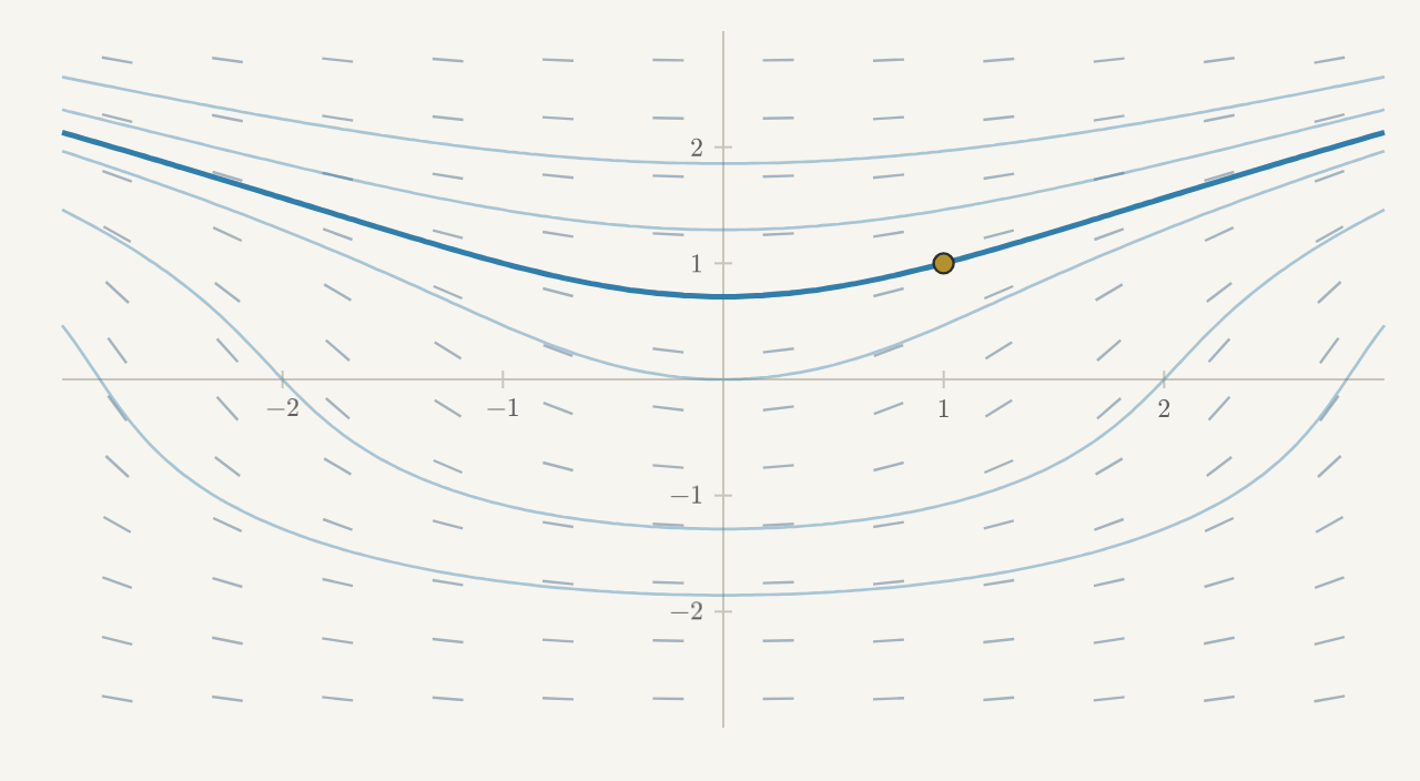
The denominator $1 + 𝑦 (𝑡) = \sqrt 𝑡 2 + 4$ never vanishes, and $𝑦 (0) = 1$ , so this formula solves the initial value problem on the whole real line.

But separation does not always leave a relationship which is useful to invert. For example, suppose

𝑦' = 𝑡 1 + 𝑦 2 .

Moving the $𝑦$ -dependent factor to the left gives

(1 + 𝑦 2) 𝑑 𝑦 = 𝑡 𝑑 𝑡 .

After integrating, we obtain

𝑦 + 𝑦 3 3 = 𝑡 2 2 + 𝐶 .

This relation specifies the solution even though we have not isolated $𝑦$ . We could use the cubic formula to do so, but the result would be much harder to read and would tell us very little. An equation relating $𝑡$ and $𝑦$ in this way is called an implicit solution, and it is every bit as exact as an explicit formula $𝑦 = 𝑓 (𝑡)$ . If we want a numerical value at a particular time, we can solve the resulting cubic numerically.

Definition 2.3 (Implicit and explicit solutions). An explicit solution gives the unknown directly as $𝑦 = 𝑓 (𝑡)$ . An implicit solution gives a relation

𝐺 (𝑡, 𝑦) = 𝐶

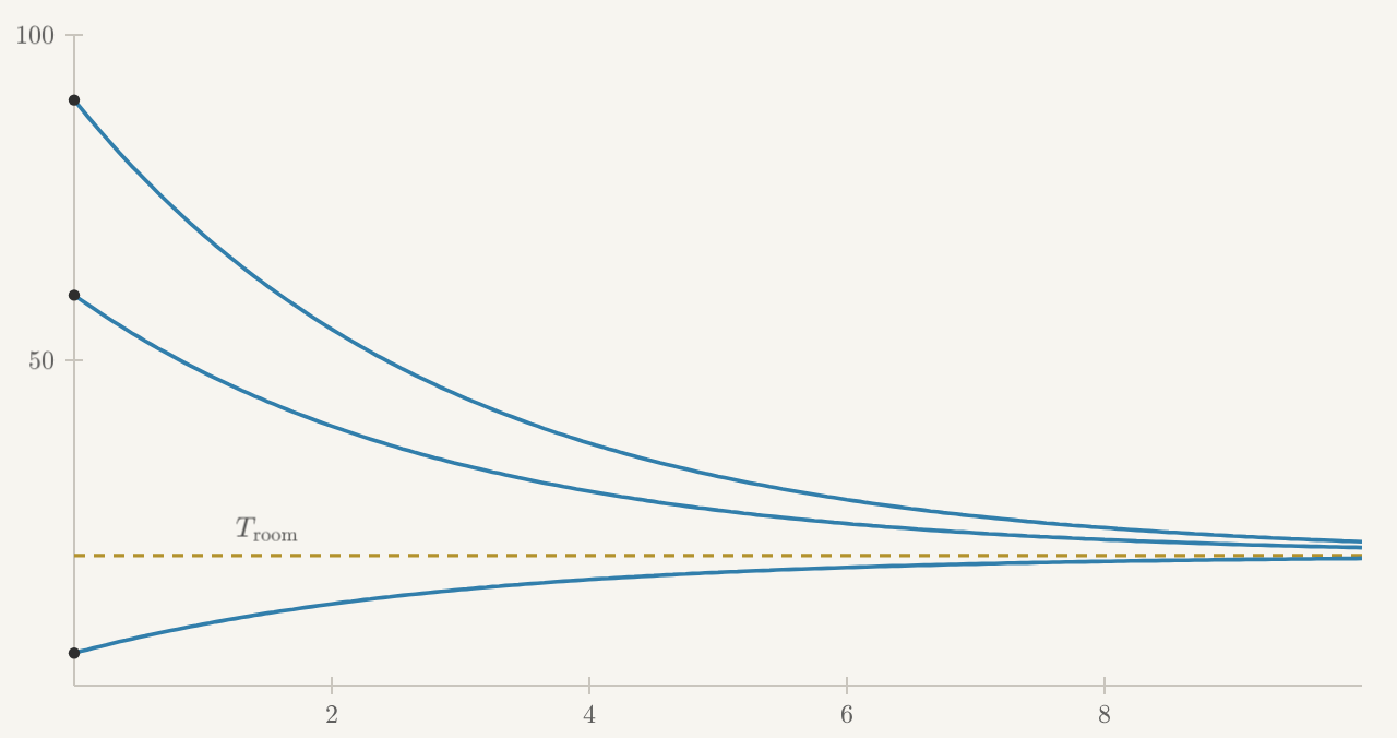
whose differentiable branches $𝑦 (𝑡)$ satisfy the differential equation. The second form is no less exact merely because $𝑦$ has not been isolated.

Figure 2.3 An implicit solution is still a curve we can draw. Each blue curve consists of the points satisfying $𝑦 + 𝑦 3 / 3 = 𝑡 2 / 2 + 𝐶$ , even though we never isolate $𝑦$ . Drag the gold point to choose an initial condition; the readout determines $𝐶$ and draws the one implicit solution through that point.

Before leaving separation, let us return to cooling. Newton's law said that the rate of change of temperature is proportional to the difference between the object's temperature and its surroundings, with $𝑘 > 0$ :

𝑇' = - 𝑘 (𝑇 - 𝑇 r o o m) .

The repeated expression $𝑇 - 𝑇 r o o m$ is the clue. Let $𝑢 = 𝑇 - 𝑇 r o o m$ be that temperature difference. Since the room temperature is constant, $𝑢' = 𝑇'$ , and the equation becomes

𝑢' = - 𝑘 𝑢 .

We can find the constant solution $𝑢 = 0$ first, and then separate the nonzero solutions:

𝑑 𝑢 𝑢 = - 𝑘 𝑑 𝑡 .

Thus $l n | 𝑢 | = - 𝑘 𝑡 + 𝐶$ . If $𝑇 (0) = 𝑇 0$ , then $𝑢 (0) = 𝑇 0 - 𝑇 r o o m$ , so $𝑢 = (𝑇 0 - 𝑇 r o o m) 𝑒 - 𝑘 𝑡$ . Returning to temperature gives

𝑇 (𝑡) = 𝑇 r o o m + (𝑇 0 - 𝑇 r o o m) 𝑒 - 𝑘 𝑡 .

Now the qualitative story we told from the local rule is visible in a single formula. The exponential factor tends toward zero, so a hot object cools toward the room temperature while a cold object warms toward it. The same equation, and the same formula, contains both stories.

Figure 2.4 Cooling, solved. Three starting temperatures ride the same formula $𝑇 (𝑡) = 𝑇 r o o m + (𝑇 0 - 𝑇 r o o m) 𝑒 - 𝑘 𝑡$ — hot mugs cooling down and a cold drink warming up are one calculation. In the live figure, drag the room-temperature line itself: every solution chases the new room temperature.

2.4Undoing the Product Rule

Separation was really the chain rule used in reverse. Can we play the same game with another familiar rule? Sometimes an equation contains the pieces of a product rule, but the product they came from has been broken apart. Consider

(1 + 𝑡 2) 𝑦' + 2 𝑡 𝑦 = 1 .

The two terms on the left look as though they came from differentiating a product. Indeed,

𝑑 𝑑 𝑡 ((1 + 𝑡 2) 𝑦) = (1 + 𝑡 2) 𝑦' + 2 𝑡 𝑦 .

So we can group the entire left-hand side into one derivative:

𝑑 𝑑 𝑡 ((1 + 𝑡 2) 𝑦) = 1 .

Now antidifferentiation gives

(1 + 𝑡 2) 𝑦 = 𝑡 + 𝐶, a n d h e n c e 𝑦 = 𝑡 + 𝐶 1 + 𝑡 2 .

Nothing new had to be invented here. We simply recognized the remains of a product rule and put the product back together.

Often the needed product is not visible until we create it. For example, look at

𝑦' + 2 𝑡 𝑦 = 2 𝑡 .

The left side is not currently the derivative of a product. Suppose we multiply the whole equation by some function $𝑚 (𝑡)$ :

𝑚 𝑦' + 2 𝑡 𝑚 𝑦 = 2 𝑡 𝑚 .

If the left side is to equal $(𝑚 𝑦)' = 𝑚 𝑦' + 𝑚' 𝑦$ , then we need the coefficient of $𝑦$ to satisfy

𝑚' = 2 𝑡 𝑚 .

We recognize one function with exactly that derivative relationship: $𝑚 (𝑡) = 𝑒 𝑡 2$ . Multiplying by it turns the equation into

𝑒 𝑡 2 𝑦' + 2 𝑡 𝑒 𝑡 2 𝑦 = 2 𝑡 𝑒 𝑡 2,

or, after putting the product back together,

𝑑 𝑑 𝑡 (𝑒 𝑡 2 𝑦) = 2 𝑡 𝑒 𝑡 2 .

Both sides can now be antidifferentiated:

𝑒 𝑡 2 𝑦 = 𝑒 𝑡 2 + 𝐶, s o 𝑦 = 1 + 𝐶 𝑒 - 𝑡 2 .

The multiplying function $𝑒 𝑡 2$ is called an integrating factor. But the name is not the point; the point is the question which produced it: what could we multiply by so that the product rule gathers several terms into one derivative?

We managed to invent the right multiplier for this equation, but was that good luck? In the next chapter we will make this construction systematic for a whole class of equations, and use it to prove that their initial value problems have exactly one solution.

First, though, we need another way to find answers. Our calculus techniques depend on recognizing a useful structure in the equation. What can we do when we do not find one? The slope field still gives us a direction at every point. Perhaps we can turn the act of following those directions into a calculation.

2.5Euler's Method

Let us try this on the initial value problem

{𝑦' = 𝑦 (1 - 𝑦) + 0.1 𝑡, 𝑦 (0) = 0.1 .

This looks suspiciously like the sort of equation we should be able to solve for homework. But the $0.1 𝑡$ prevents us from separating the variables, and there is no product rule on the left waiting to be put back together. None of the calculus techniques we have developed gives us a formula.

Still, the differential equation answers one small question perfectly. At the initial point $(0, 0.1)$ , it tells us the slope:

𝐹 (0, 0.1) = 0.1 (1 - 0.1) + 0.1 (0) = 0.09 .

What can we do with one slope? The tangent-line approximation says that for a short time $ℎ$ , the change in $𝑦$ should be approximately

c h a n g e i n 𝑦 \approx ℎ (0.09) .

If we take $ℎ = 1$ , this predicts a new value

𝑦 1 = 0.1 + 1 (0.09) = 0.19 .

Of course, there is no reason to keep trusting the old slope once we arrive at this new point. So we do something much more sensible: ask the differential equation again! It gives us the slope at $(1, 0.19)$ , we follow that slope for another short step, and then we ask again. The equation supplies the local rule; our computation repeatedly checks in with it as the state changes.

In general, if our current approximation is $(𝑡 𝑛, 𝑦 𝑛)$ , this repeated conversation becomes Euler's method.

Definition 2.4 (Euler's method). For the initial value problem $𝑦' = 𝐹 (𝑡, 𝑦)$ , $𝑦 (𝑡 0) = 𝑦 0$ , choose a step size $ℎ$ . Starting from $(𝑡 0, 𝑦 0)$ , Euler's method produces successive approximations by

𝑡 𝑛 + 1 = 𝑡 𝑛 + ℎ, 𝑦 𝑛 + 1 = 𝑦 𝑛 + ℎ 𝐹 (𝑡 𝑛, 𝑦 𝑛) .

There is nothing more hidden in the method: it is the familiar tangent-line approximation, restarted over and over. Continuing our $ℎ = 1$ calculation by hand gives

𝑛 𝑡 𝑛 𝑦 𝑛 𝐹 (𝑡 𝑛, 𝑦 𝑛) 𝑦 𝑛 + 1 00 0.100 0.090 0.190 11 0.190 0.254 0.444 22 0.444 0.447 0.891

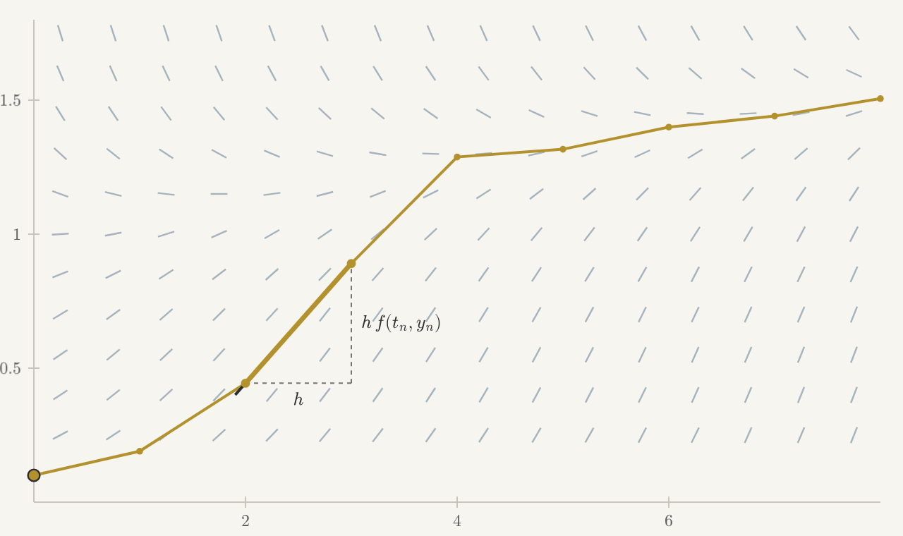
There is something important hiding in this little table. The values $𝑦 𝑛$ are not points sampled from a solution we secretly know. They are the approximations we have produced so far, and each new slope is evaluated at one of those approximate points. The computation builds the history and uses the history it has built to decide what to do next.

Figure 2.5 Euler's method turns local slopes into a polygonal history. Each segment borrows the slope at its left endpoint: $ℎ$ units across and $ℎ 𝐹 (𝑡 𝑛, 𝑦 𝑛)$ units up. Smaller steps ask the equation for new information more often and bend through the field more faithfully. In the live figure, click a step to inspect it, change $ℎ$ , play the construction, or drag the initial point.

The step size $ℎ$ answers a practical question: how long are we willing to trust one tangent line? With $ℎ = 1$ , we travel fairly far before checking the rule again. With $ℎ = 0.2$ , we ask five times as often. This costs five times as many slope calculations, but the smaller-step polygons in the figure appear to settle toward a common curve. That is good evidence that we are finding the solution---though it is not yet a proof.

The method is quite easy to translate into code. The following Python loop says exactly what we just said: ask for a slope, use it to update the value, update the time, and repeat.

def euler(F, t0, y0, h, steps):
    t = t0
    y = y0
    points = [(t, y)]

    for _ in range(steps):
        y = y + h * F(t, y)
        t = t + h
        points.append((t, y))

    return points


def F(t, y):
    return y * (1 - y) + 0.1 * t


points = euler(F, 0, 0.1, 0.5, 16)

The list points is the polygon drawn in the figure. There is no hidden solver inside the code. This tiny loop is the solver.

Earlier, a Riemann sum gave us a way to approximate the accumulated change when the rate was a known function of time. Euler's method has extended that idea to a rate which depends on the unknown value as well. To see this, add up the first $𝑛$ updates:

𝑦 𝑛 = 𝑦 0 + 𝑛 - 1 \sum 𝑘 = 0 ℎ 𝐹 (𝑡 𝑘, 𝑦 𝑘) .

If $𝐹 (𝑡, 𝑦) = 𝑔 (𝑡)$ does not depend on $𝑦$ , this is an ordinary left Riemann sum for $\int 𝑔 (𝑡) 𝑑 𝑡$ : all the rates can be known before the sum begins. In general, each rate $𝐹 (𝑡 𝑘, 𝑦 𝑘)$ depends on the value the sum has reached so far. Euler's method is a Riemann sum which learns what to add next from its own running total.

How much should we trust the result? We can test the method on equations we already know how to solve, and we can repeat a computation with smaller and smaller values of $ℎ$ to see whether the answers agree. Both are useful evidence. Neither, by itself, guarantees that an arbitrary computation is accurate. Building that guarantee requires a mathematical theory of error and stability, which we will develop when we study how to trust a computed trajectory. For now, Euler's method gives us the central idea on which much more powerful numerical solvers are built: follow the local rule for a short time, then ask again.

We can now find solutions in several ways. A remembered function may give us a successful guess; a calculus rule may reconstruct an exact answer; a sequence of short steps may give us a useful numerical approximation. But these methods also leave us with questions.

If we cannot find a formula, is there nevertheless a solution to find? If we have checked one, could there be another with the same initial condition? And how far in time does the solution continue? Euler's update lets us ask for another step, but that alone does not tell us whether an exact solution exists at the time we are trying to reach.

These are questions about the differential equation itself, whether or not we can solve it explicitly. In the next chapter we will begin answering them.

Problems

The routine problems ask you to guess and check, use calculus to find solutions, and step numerically with Euler’s method. In the Python problems, begin with the supplied structure and make the computation your own.

Check Your Understanding

1Exponentials turn calculus into algebra

For each equation, try $𝑦 = 𝑒 𝑟 𝑡$ , determine every value of $𝑟$ which works, and verify the resulting functions by substitution.

(a)

$𝑦 ″ - 𝑦' - 6 𝑦 = 0$ .

(b)

$𝑦 ‴ + 𝑦 ″ - 4 𝑦' - 4 𝑦 = 0$ .

(c)

The three exponential solutions you found for the third-order equation all satisfy $𝑦 (0) = 1$ . Calculate their values of $𝑦' (0)$ and $𝑦 ″ (0)$ . Does specifying only $𝑦 (0)$ distinguish these solutions?

2A spring with a different clock

Consider $𝑥 ″ = - 9 𝑥$ .

(a)

Motivate a trigonometric guess, then verify that $𝑥 (𝑡) = 𝐴 c o s (3 𝑡) + 𝐵 s i n (3 𝑡)$ solves the equation for every $𝐴$ and $𝐵$ .

(b)

Choose $𝐴$ and $𝐵$ so that $𝑥 (0) = 2$ and $𝑥' (0) = - 6$ .

(c)

What is the period of this motion? Check your answer directly from the formula rather than quoting a memorized spring formula.

3Accumulating a known rate

Solve each initial value problem exactly. Give an integral-defined answer when an elementary antiderivative is not available.

(a)

$𝑦' = 3 𝑡 2 - 4 𝑡 + 1$ , $𝑦 (1) = 2$ .

(b)

$2 𝑦' + 6 𝑡 = 4$ , $𝑦 (- 1) = 0$ .

(c)

$𝑦' = 𝑒 - 𝑡 2$ , $𝑦 (0) = 3$ . Then explain what the Fundamental Theorem of Calculus lets you know about your answer even though you cannot simplify its integral.

4Separate carefully

For each equation, find every constant solution before dividing, then find the remaining solutions and impose the initial condition.

(a)

$𝑦' = 𝑡 (1 - 𝑦)$ , $𝑦 (0) = 3$ .

(b)

$𝑦' = 𝑦 (2 - 𝑦)$ , $𝑦 (0) = 1$ .

(c)

In the previous part, identify the step which would have discarded two solutions if you had performed it too early.

5An implicit solution is still a solution

Separate $𝑦' = 𝑡 / (1 + 𝑦 4)$ with $𝑦 (0) = 1$ . Leave your answer as an implicit relation. Differentiate that relation with respect to $𝑡$ to verify that its branches satisfy the original differential equation.

6Put the product back together

Solve each equation by recognizing or creating a product derivative.

(a)

$(1 + 𝑡) 𝑦' + 𝑦 = 𝑡 2$ on an interval which does not contain $𝑡 = - 1$ .

(b)

$𝑦' + 3 𝑡 2 𝑦 = 3 𝑡 2$ , using the integrating factor $𝑒 𝑡 3$ .

(c)

Check the family you found in the previous part by substitution. Which member is the constant solution?

7Euler by hand

Apply Euler's method to $𝑦' = 𝑡 - 𝑦$ , $𝑦 (0) = 1$ .

(a)

With $ℎ = 0.5$ , build a table through $𝑡 = 2$ containing $𝑡 𝑛$ , $𝑦 𝑛$ , the sampled slope, and $𝑦 𝑛 + 1$ .

(b)

The exact solution is $𝑦 = 𝑡 - 1 + 2 𝑒 - 𝑡$ . Compare your approximation at $𝑡 = 2$ with the exact value.

(c)

Without recomputing, point to the entries of your table which show that Euler's method used its own approximate history to choose later slopes.

Explorations

8One equation, two methods

Consider

𝑦' + 2 𝑡 𝑦 = 2 𝑡 .

(a)

Rewrite the equation in separable form. First find any constant solutions. Then separate variables on intervals where the factor you divide by is nonzero, and solve.

(b)

Solve the same equation by multiplying by $𝑒 𝑡 2$ and recognizing a product derivative.

(c)

Show that your two answers describe the same family, even if their constants look different. Which solution needed separate attention during separation? How does it appear in the product-rule answer?

(d)

Use either answer to find a solution satisfying $𝑦 (0) = 3$ , and check it directly.

9Choosing a branch

Consider the equation

𝑦' = 𝑡 1 + 𝑦

with two different initial conditions:

𝑦 (2) = 0 a n d 𝑦 (2) = - 2 .

(a)

Separate and integrate for each initial condition. Show that both lead to the same implicit relation

(𝑦 + 1) 2 = 𝑡 2 - 3 .

(b)

Solve this relation for $𝑦$ . Which branch satisfies each initial condition? Differentiate both formulas to check the differential equation.

(c)

For each answer, find the largest open interval containing $𝑡 = 2$ on which the formula satisfies the original equation. What happens to $𝑦$ as $𝑡$ approaches the left endpoint? Why can't that endpoint be included, even though the formula has a finite value there?

(d)

The formulas also give real values when $𝑡 < - \sqrt 3$ . Explain why those values do not extend either solution through the intervening gap.

Python: From a Loop to Evidence

10Write Euler's method once

Complete the two missing update lines in this function.

def euler(F, t0, y0, h, steps):
    t = t0
    y = y0
    ts = [t]
    ys = [y]

    for _ in range(steps):
        # update y using the slope at the old point
        # update t
        ts.append(t)
        ys.append(y)

    return ts, ys

(a)

Test your function on $𝑦' = 𝑦$ , $𝑦 (0) = 1$ through $𝑡 = 2$ , using step sizes $ℎ = 0.5$ , $0.25$ , and $0.125$ . Plot all three polygons with $𝑒 𝑡$ on the same axes.

(b)

For each step size, compute the absolute error at $𝑡 = 2$ . Put the results in a small table. What happens to the error when $ℎ$ is halved?

(c)

Change the right-hand side to $𝐹 (𝑡, 𝑦) = 𝑦 (1 - 𝑦) + 0.1 𝑡$ . Which lines of your solver change, and which do not? Explain why that separation is useful.

11Plot an implicit family

The separated equation in figure 2.3 produced the family $𝑦 + 𝑦 3 / 3 = 𝑡 2 / 2 + 𝐶$ .

Use numpy.linspace to make grids of $𝑡$ and $𝑦$ , evaluate

G = Y + Y**3 / 3 - T**2 / 2

on the grid, and use plt.contour(T, Y, G, levels=[...]) to draw at least five values of $𝐶$ . Mark one initial point, compute its value of $𝐶$ , and highlight the corresponding contour. Explain why a contour plot can draw the exact family without ever solving explicitly for $𝑦$ .