Chapter 1

What is a Differential Equation

This course is about differential equations. But what is a differential equation? We are all familiar with algebraic equations, where there is an unknown number (say x) satisfying some relationship involving the operations of algebra, like $𝑥 2 + 4 𝑥 = 5$ . And solving an algebraic equation means to find the value(s) of $𝑥$ that actually realize this relationship.

A differential equation is a similar type of object, but for calculus. The unknown is no longer a number, but rather a function (say $𝑓$ ), and the relationship can involve the operations of calculus, like $𝑓'' + 4 𝑓' = 5 𝑓$ . Solving a differential equation means finding the function(s) which actually have this relationship with one another.

There are many superficial similarities between differential equations, and the algebraic case you already know. Just like polynomials can come in many different degrees like $𝑥 + 2 = 5$ of $𝑥 2 - 3 𝑥 + 2 = 0$ or $𝑥 5 - 3 𝑥 3 = 2$ , differential equations come in different orders, where the order is defined as the highest derivative showing up in the equation. So $𝑓'' = 4 𝑓$ is a second order equation, and $𝑑 3 𝑑 𝑥 3 𝑦 = 4 𝑦 + 𝑒 𝑥$ is third order. And like algebraic equations, they can also come in systems: the two algebraic equations

𝑥 + 𝑦 = 3, 𝑥 - 𝑦 = 1

form a system for the two unknown numbers $𝑥$ and $𝑦$ . A system of differential equations asks the same thing of unknown functions. For example,

𝑓' = 𝑔, 𝑔' = - 𝑓

is a system for the two unknown functions $𝑓$ and $𝑔$ . The solution to this system is then a pair of functions: after thinking about the system a bit, can you see what a solution could be?

Like in algebra, checking a solution works is easy: if I give you $𝑥 = 1$ or $𝑥 = - 5$ you can directly plug them into the equation and observe you get the same thing on both sides. And, if I give you $𝑓 = 𝑒 𝑡$ or $𝑓 = 𝑒 - 5 𝑡$ , you can differentiate, plug into the differential equation, and see that each side gives you the same function.

In both cases the theory of how to find these solutions is more involved: even though you learn the rules of arithmetic in elementary school you don't learn to solve algebraic equations until high school. And similarly for differential equations: you leanred the rules of differentiation in Calculus, but now its finally our time to put them to use!

1.1Local Rules

It's not really that much of an exaggeration to say that differential equations run the world. From economic models, across engineering and the sciences, to our best theories of fundamental physics, all are phrased in the language of differential equations. Perhaps much of this stems from the great mystery that our universe is so well described by mathematics. But there is also a practical, human reason that differential equations show up so often in our lives: it is usually much easier to describe what is happening right now than to describe the whole future at once.

The derivative is exactly this sort of local information. If $𝑦 (𝑡)$ records some quantity which is changing over time, then $𝑦' (𝑡)$ tells us how it is changing near one particular instant. For a small step $ℎ$ ,

𝑦 (𝑡 + ℎ) \approx 𝑦 (𝑡) + ℎ 𝑦' (𝑡) .

Thus, an equation like

𝑦' = 𝐹 (𝑡, 𝑦)

is a rule for how the function should behave nearby each point: if we know the current time $𝑡$ and the current value $𝑦$ , the right hand side tells us the current rate of change. The function $𝑦 (𝑡)$ is the unknown history; $𝐹 (𝑡, 𝑦)$ is the known local rule.

This is often exactly the kind of knowledge the world gives us. Imagine a hot cup of coffee sitting in a room. It may be difficult to say immediately what its temperature will be twenty minutes from now. But it is easy to say how its temperature is changing now: a cup hotter than the room cools down, a cup colder than the room warms up, and a larger temperature difference produces a faster change. The simplest rule with these properties is

𝑇' = - 𝑘 (𝑇 - 𝑇 r o o m), 𝑘 > 0 .

Our simple observation about the rate of heating and cooling, translated into mathematics, gives a differential quation for the temperature $𝑇$ . And if we learn to solve such equations (giving us a function $𝑇 (𝑡)$ ) we will have the answer to our original question - how cool will the coffee be in 20 minutes - without any more input from physics at all. Differential equations allow us to package together simple relational information, and solving them integrates all these local relationships into a global story.

The same idea works when several things are changing together. It is hard to predict the complete histories of a population of hares and a population of lynx. But some local relationships are easy to express: more hares mean more food for lynx, while more lynx mean more encounters in which hares are eaten. This seems like almost no information, yet thinking slowly through how to express this precisely (which we will do in the next chapter) allows one to write down a rather simple set of expressions for the rate of change $𝐻'$ of the number of hares, and $𝐿'$ for the number of Lynx, in terms of their current populations:

𝐻' = 𝑟 𝐻 - 𝑏 𝐻 𝐿, 𝐿' = 𝑐 𝐻 𝐿 - 𝑑 𝐿 .

Neither population can now be understood by itself: their two local rules are coupled.

Or consider a mass attached to a spring. The farther the spring is stretched, the harder it pulls back. A simplest precise verison of this would say that the force it pulls with is proportional to the stretch distance $𝑥$ . and Newton's law turns force into acceleration:

𝑚 𝑥 ″ = - 𝑘 𝑥 .

None of these local rules tells us the complete history all at once. A solution is an overall function—or collection of functions—which obeys the rule at every point. It integrates all those nearby instructions into one coherent relationship. This is the reversal at the heart of differential equations: differentiation begins with a known history and extracts its local behavior; a differential equation begins with the local behavior and asks us to reconstruct the possible histories.

We can now collect this language precisely.

Definition 1.1 (Differential equations and solutions). A differential equation is an equation whose unknown is a function and which relates that function to one or more of its derivatives. Its order is the order of the highest derivative which appears.

A solution on an interval is a function which has the required derivatives and makes the equation true at every time in that interval. If several unknown functions must satisfy several differential equations together, the equations form a system, and a solution is the corresponding collection of functions.

1.2Slope Fields

In algebra it is useful to have a graph to help conceptualize a problem (say for a quadratic equation, you can immediately see how many roots there'll be if you can draw a picture, even if you haven't exactly sovled for them yet). And we might hope to find an analog for differetial equations - somethign we can draw that will tell us how thigns behave, even if we haven't done all the work of producing an exact solution yet.

But what's the graph of a differential equation? For the moment, let's focus on the simplest general case: one unknown function $𝑦 (𝑡)$ and one first-order equation

𝑦' = 𝐹 (𝑡, 𝑦) .

In algebra, we dont draw the number $𝑥$ but the relationship $𝑦 = 𝑓 (𝑥)$ . Similarly here we cant draw the function $𝑦 (𝑡)$ (since we don't know it yet!) but we will try to draw the relationship itself. This relationship is given to us by a function $𝐹 (𝑡, 𝑦)$ which we can compute at any point $(𝑡 0, 𝑦 0)$ . Since this is equal to $𝑦'$ , the relationship tells us nothing about the value, but rather it answers the question

If a solution passes through $(𝑡 0, 𝑦 0)$ , what slope must it have there?

For example, consider

𝑦' = 𝑡 - 𝑦 .

If a solution passes through $(1, - 1)$ , its slope there must be

𝑦' = 1 - (- 1) = 2 .

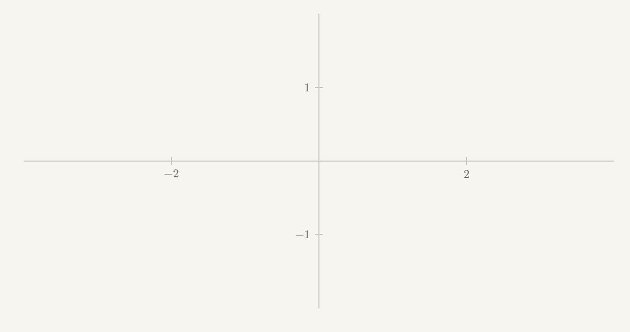
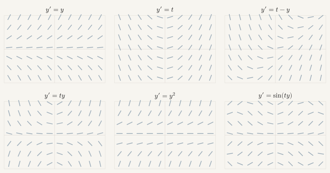
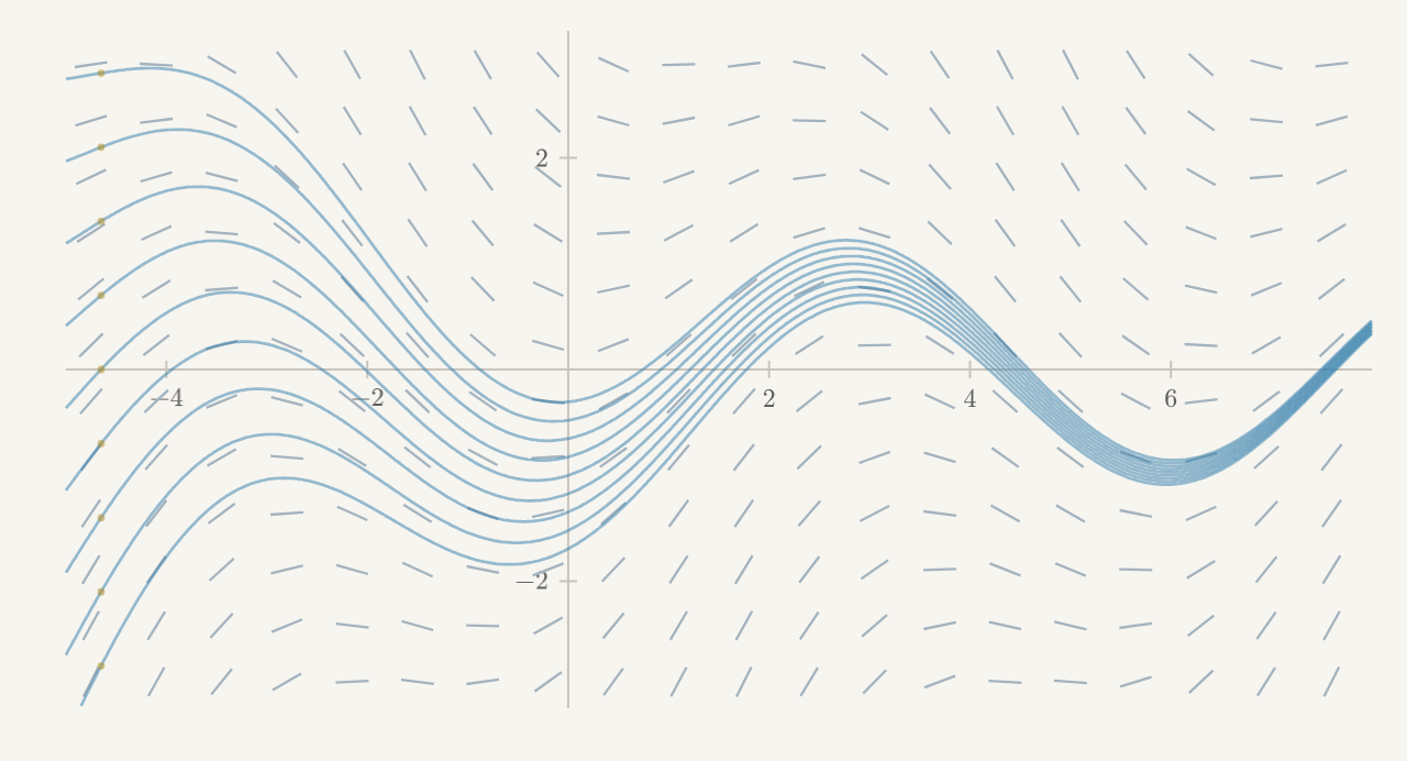
Thus we do not know the solution, but we know one of its tangent lines! We can record that information by drawing a tiny line segment of slope $2$ at the point $(1, - 1)$ . Of course there is nothing special about this point. We can ask the same question at every other point in the plane and draw the answer there too.

Figure 1.1 The slope field of $𝑦' = 𝑡 - 𝑦$ . At each point the equation answers one small question: if a solution passed through here, what slope would it have? The field is that question asked everywhere — pure evaluation, no solving. In the live figure, move over the plane to ask the equation yourself, click to leave a slope behind, and try to draw a solution one slope at a time before revealing the field. (Draft caption — final wording at prose stage.)

The result is called a slope field. We have evaluated the rule everywhere, but we have not solved the equation. Different equations paint very different pictures. Some fields repeat their slopes along horizontal lines, others along vertical lines; some push curves away from the axis, while others pull them toward it. But every one of them is constructed and read in exactly the same way: evaluate the right hand side, then draw the resulting slope.

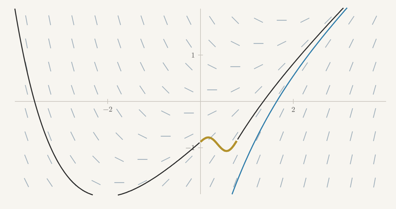
Figure 1.2 Six equations, six personalities. Every field is read the same way — flat ticks where $𝑦' = 0$ , steep ticks where the rule demands speed — but each equation paints its own portrait. (Draft caption — final wording at prose stage.)

What does a solution look like in this picture? A function $𝑦 (𝑡)$ is a solution precisely when its graph follows the field everywhere it goes. At each point $(𝑡, 𝑦 (𝑡))$ on the graph, the curve's own slope $𝑦' (𝑡)$ must equal the slope $𝐹 (𝑡, 𝑦 (𝑡))$ prescribed by the equation.

This is an everywhere requirement. A curve can follow the field perfectly for a long time and then make one wrong turn; at the point of that turn, it is not a solution. A function does not earn partial credit from the differential equation.

Figure 1.3 A solution and an impostor. The blue curve follows the field everywhere it goes. The other curve is a real solution on its dark stretches — but no single solution connects them, so the highlighted stretch is forced to disobey: watch it cut across the ticks. Being a solution is a pointwise obligation, and the failure has a location. In the live figure, click or drag anywhere to move the blue solution through that point; it remains tangent to the field everywhere. (Draft caption — final wording at prose stage.)

This pictorial description already has taught us something important: there is not just one solution to a differential equation. The slope field is filled by an entire family of curves, each following the same local rule. To choose one of them, we specify one piece of additional information: the value of the function at some time. Writing

𝑦 (𝑡 0) = 𝑦 0

says that our solution must pass through the point $(𝑡 0, 𝑦 0)$ . This is called an initial condition, and the equation together with this condition is called an initial value problem:

𝑦' = 𝐹 (𝑡, 𝑦), 𝑦 (𝑡 0) = 𝑦 0 .

The differential equation describes the possible histories; the initial condition specifies a point the history must pass through.

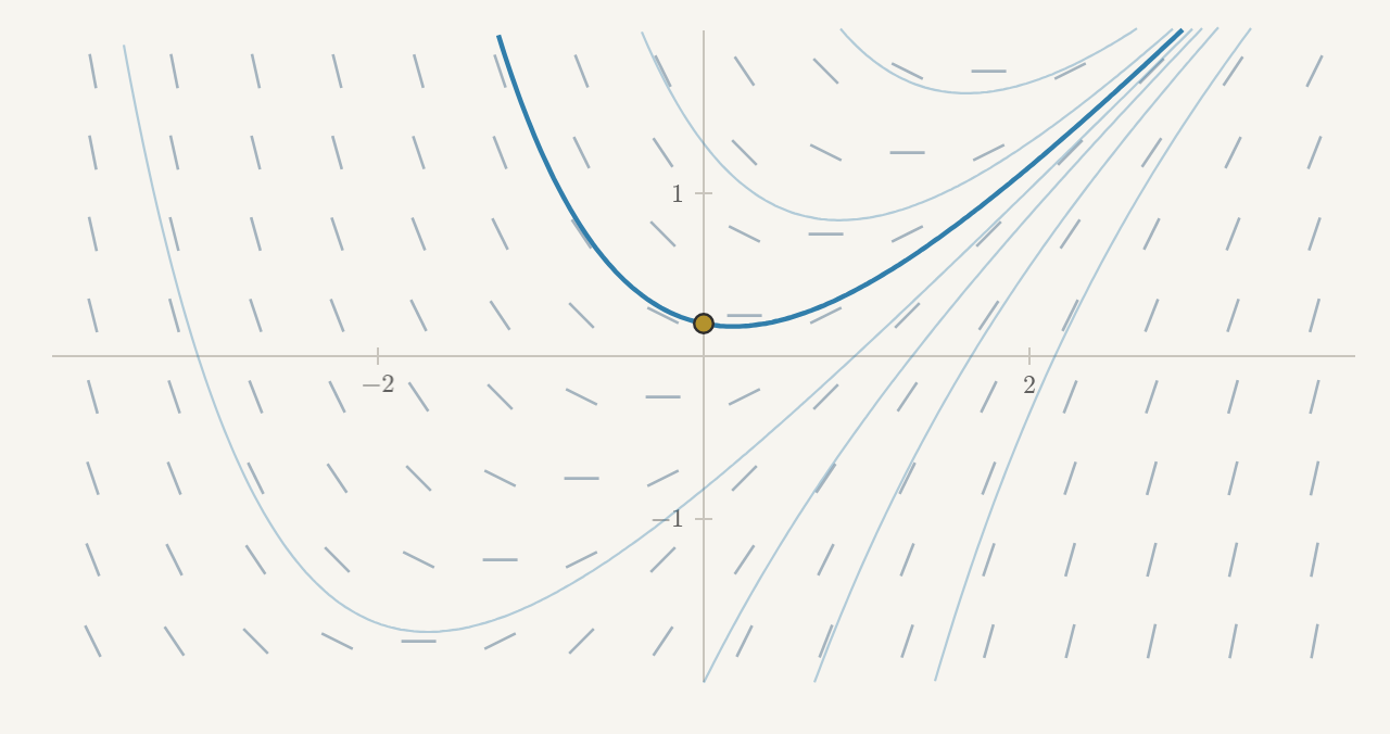
Definition 1.2 (Initial conditions and initial value problems). An initial condition specifies the value of an unknown function at a chosen time, such as $𝑦 (𝑡 0) = 𝑦 0$ . An initial value problem consists of a differential equation together with initial conditions prescribed at one time. A solution of the initial value problem must satisfy both the equation and all of the initial conditions.

Figure 1.4 The gold point is an initial condition $𝑦 (𝑡 0) = 𝑦 0$ . In this figure, each starting point selects one member of the displayed solution family. Follow its curve in both time directions and compare its tangent with the field. In the live figure, click or drag to move the data. (Draft caption — final wording at prose stage.)

The slope field does tell us one thing about how solution curves can meet. At each point, the equation prescribes just one slope. If two solutions pass through the same point, they must have the same tangent there. They cannot meet with different tangents.

But could two curves meet with the same tangent and then separate? Does an initial condition always select exactly one solution, and how far can we follow it? We will investigate these questions in chapter 3. For now, we can explore the histories suggested by the slope field.

Even without a formula for a single solution, a slope field can tell us where solutions rise and fall, where they have horizontal tangents, and how different starting points may lead to different futures. This is genuine information about the unknown functions, extracted directly from the differential equation.

Try turning the local picture into a global one yourself. Each time you choose a point, the differential equation supplies the slopes which carry one solution through it. Add enough starting points and the slope field begins to fill with histories: the local rule becomes a flow.

Figure 1.5 Build the flow. Click anywhere to add the complete solution through that point, or drag across the field to paint many solutions at once. Compare the blue histories with the slopes prescribed along them. Use the menu to change the local rule: the streams may gather, spread, or divide into horizontal bands, but every curve is still assembled from the slopes it meets. (Draft caption — final wording at prose stage.)

1.3Slope Fields with More Variables

So far our slope fields have described equations with one unknown function, $𝑦 (𝑡)$ . But we began this chapter with systems involving several unknown functions at once. What should a slope field look like for a system such as

{𝑓' = 𝐹 (𝑡, 𝑓, 𝑔), 𝑔' = 𝐺 (𝑡, 𝑓, 𝑔) ?

A solution is now a pair of functions, $𝑓 (𝑡)$ and $𝑔 (𝑡)$ . To graph them together, we need one axis for $𝑡$ , one for $𝑓$ , and one for $𝑔$ . Thus the graph of the solution is a curve in $(𝑡, 𝑓, 𝑔)$ -space:

𝛾 (𝑡) = (𝑡, 𝑓 (𝑡), 𝑔 (𝑡)) .

And what does the differential equation tell us at a possible point $(𝑡, 𝑓, 𝑔)$ ? It gives the two rates $𝐹 (𝑡, 𝑓, 𝑔)$ and $𝐺 (𝑡, 𝑓, 𝑔)$ . If time moves forward by a small amount $Δ 𝑡$ , then $𝑓$ changes by approximately $𝐹 Δ 𝑡$ and $𝑔$ changes by approximately $𝐺 Δ 𝑡$ . The total displacement is therefore $Δ 𝑡 (1, 𝐹, 𝐺)$ , so the system assigns the direction

(1, 𝐹 (𝑡, 𝑓, 𝑔), 𝐺 (𝑡, 𝑓, 𝑔)) .

This is exactly the slope-field idea again, only with one more component. We evaluate the equation at many possible points and draw a small segment in the direction it prescribes. The page has become a three-dimensional box, but the thought has not changed.

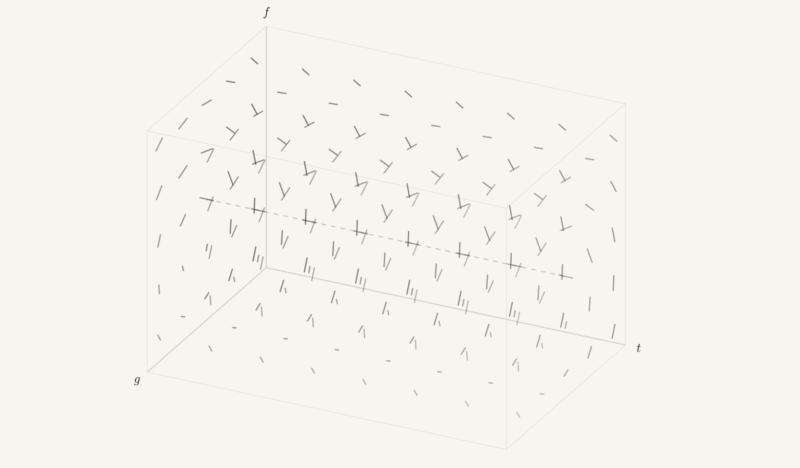
Figure 1.6 The slope field of the system $𝑓' = 𝑔$ , $𝑔' = - 𝑓$ , drawn in $(𝑡, 𝑓, 𝑔)$ -space. At each point the system prescribes one direction — one step of time, $𝑓'$ steps of $𝑓$ , $𝑔'$ steps of $𝑔$ — and the field is that answer drawn everywhere: the system itself, drawn. In the live figure, click near a tick to grow the integral curve through that point, drag to rotate, and switch to the damped sibling. (Draft caption — final wording at prose stage.)

The figure uses the system

𝑓' = 𝑔, 𝑔' = - 𝑓,

which appeared near the beginning of the chapter. Its segment at $(𝑡, 𝑓, 𝑔)$ points in the direction $(1, 𝑔, - 𝑓)$ . Clicking a segment asks for the solution through that point, and the curve grows by following one prescribed direction after another.

This also tells us exactly what it means for a pair of functions to solve a system. Along its graph,

𝛾' (𝑡) = (1, 𝑓' (𝑡), 𝑔' (𝑡)) = (1, 𝐹 (𝑡, 𝑓 (𝑡), 𝑔 (𝑡)), 𝐺 (𝑡, 𝑓 (𝑡), 𝑔 (𝑡))),

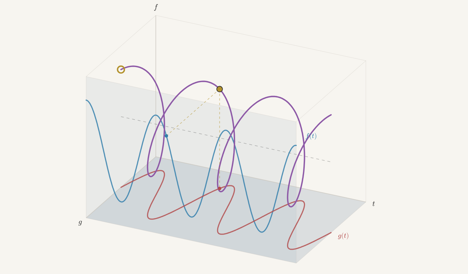
so the curve is tangent to the field everywhere it goes. An initial condition must now specify both unknowns, say $𝑓 (𝑡 0) = 𝑓 0$ and $𝑔 (𝑡 0) = 𝑔 0$ . That one point $(𝑡 0, 𝑓 0, 𝑔 0)$ again chooses one entire history.

Figure 1.7 A solution of a system is a curve in space. The violet curve solves $𝑓' = 𝑔$ , $𝑔' = - 𝑓$ ; its shadows on the wall and floor are the graphs of the two unknowns — a pair of waves, one lagging the other. The dashed line it winds around is the equilibrium solution. In the live figure, drag to rotate, drag the gold ring to move the initial condition, and switch to the damped sibling, whose curve corkscrews in toward the axis. (Draft caption — final wording at prose stage.)

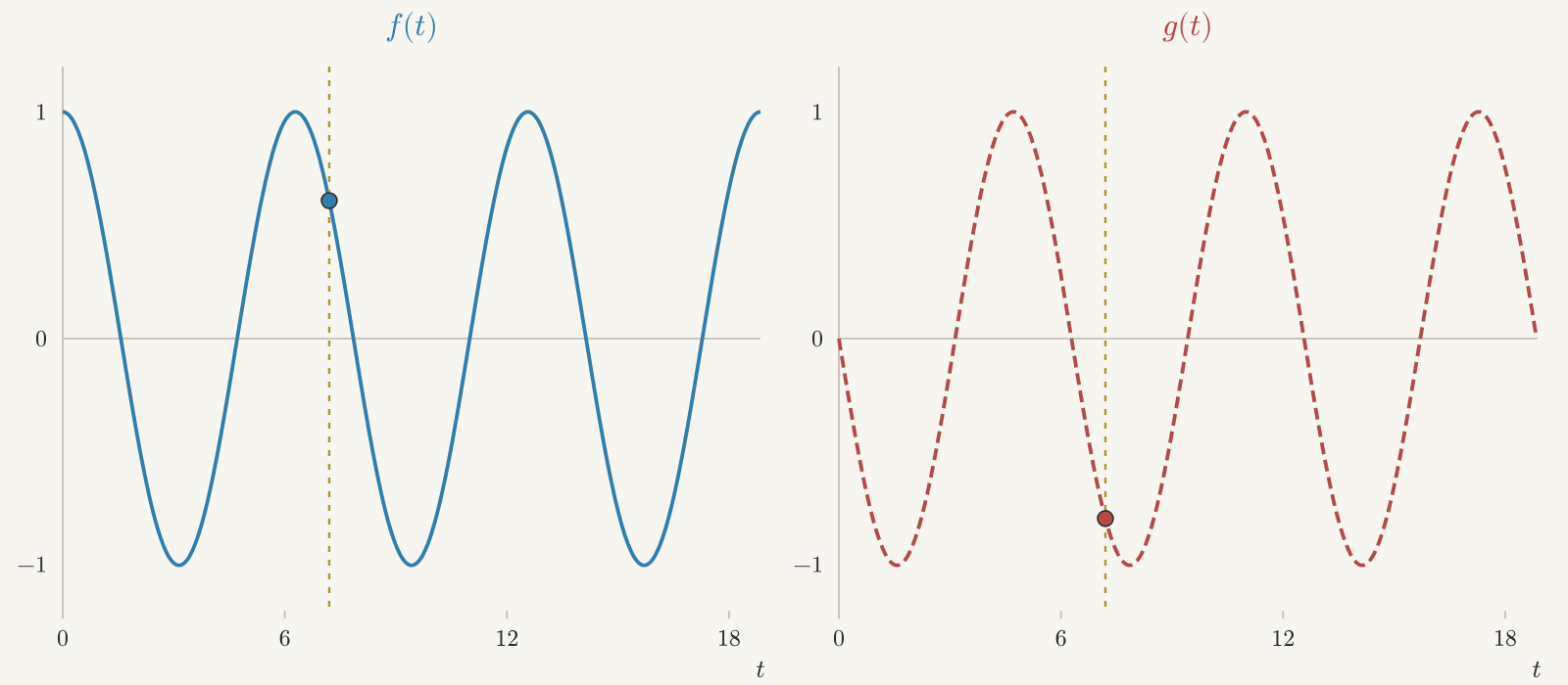
The two shadows give us another way to draw the solution: put the graph of $𝑓 (𝑡)$ beside the graph of $𝑔 (𝑡)$ . We will often display solutions this way, since ordinary graphs make it easy to read values and compare how the functions change.

Figure 1.8 The two component graphs, with points marking the same time. Together they show one solution of $𝑓' = 𝑔$ , $𝑔' = - 𝑓$ , with $𝑓 (0) = 1$ and $𝑔 (0) = 0$ .

These are two functions belonging to one solution of the system. At each time, we need both values to know what happens next. The equation $𝑓' = 𝑔$ tells us that the slope of the first graph is the height of the second; $𝑔' = - 𝑓$ tells us that the slope of the second is the negative of the height of the first.

We can therefore still read the differential equations in these pictures, but we can no longer draw the full slope field in either panel. A point $(𝑡, 𝑓)$ leaves out $𝑔$ , which we need to determine the slope. The three-dimensional picture held all that information at one point; here we have to look at the two graphs together.

This way of plotting solutions also works when there are more unknowns. For example, a simple model of an epidemic tracks three fractions of a population: the susceptible $𝑆 (𝑡)$ , the infectious $𝐼 (𝑡)$ , and the recovered $𝑅 (𝑡)$ . One such model is

𝑆' = - 𝛽 𝑆 𝐼, 𝐼' = 𝛽 𝑆 𝐼 - 𝛾 𝐼, 𝑅' = 𝛾 𝐼,

where $𝛽, 𝛾 > 0$ describe the rates of infection and recovery. We will build this model from its assumptions in chapter 4. For now, look at what a solution consists of: three functions whose derivatives satisfy these three equations together.

Figure 1.9 $𝑆 (𝑡)$ , $𝐼 (𝑡)$ , and $𝑅 (𝑡)$ on shared axes, with a common time marker. The three curves show one constructed solution of the system.

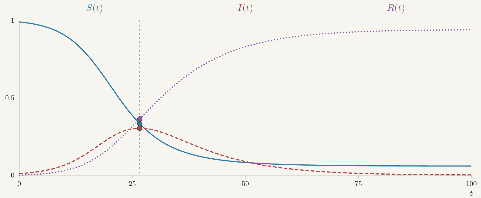
The combined graph $(𝑡, 𝑆 (𝑡), 𝐼 (𝑡), 𝑅 (𝑡))$ would use four coordinates. But we can easily draw the three functions against time. Here they share the same units, so we have placed them on the same axes. At the marked time, reading all three curves gives one snapshot of the epidemic.

Definition 1.3 (States and state spaces). The state at a particular time is the complete collection of current values which must be prescribed as initial data at that time. The set of all possible states is the state space. The individual values making up a state are its state coordinates.

For a famous example, here is a solution of the Lorenz system, drawn both as three functions of time and as the parametric curve $(𝑥 (𝑡), 𝑦 (𝑡), 𝑧 (𝑡))$ in three-dimensional space.

Figure 1.10 The marked values on the three time graphs give the coordinates of the gold point on the space curve, all at the same time.

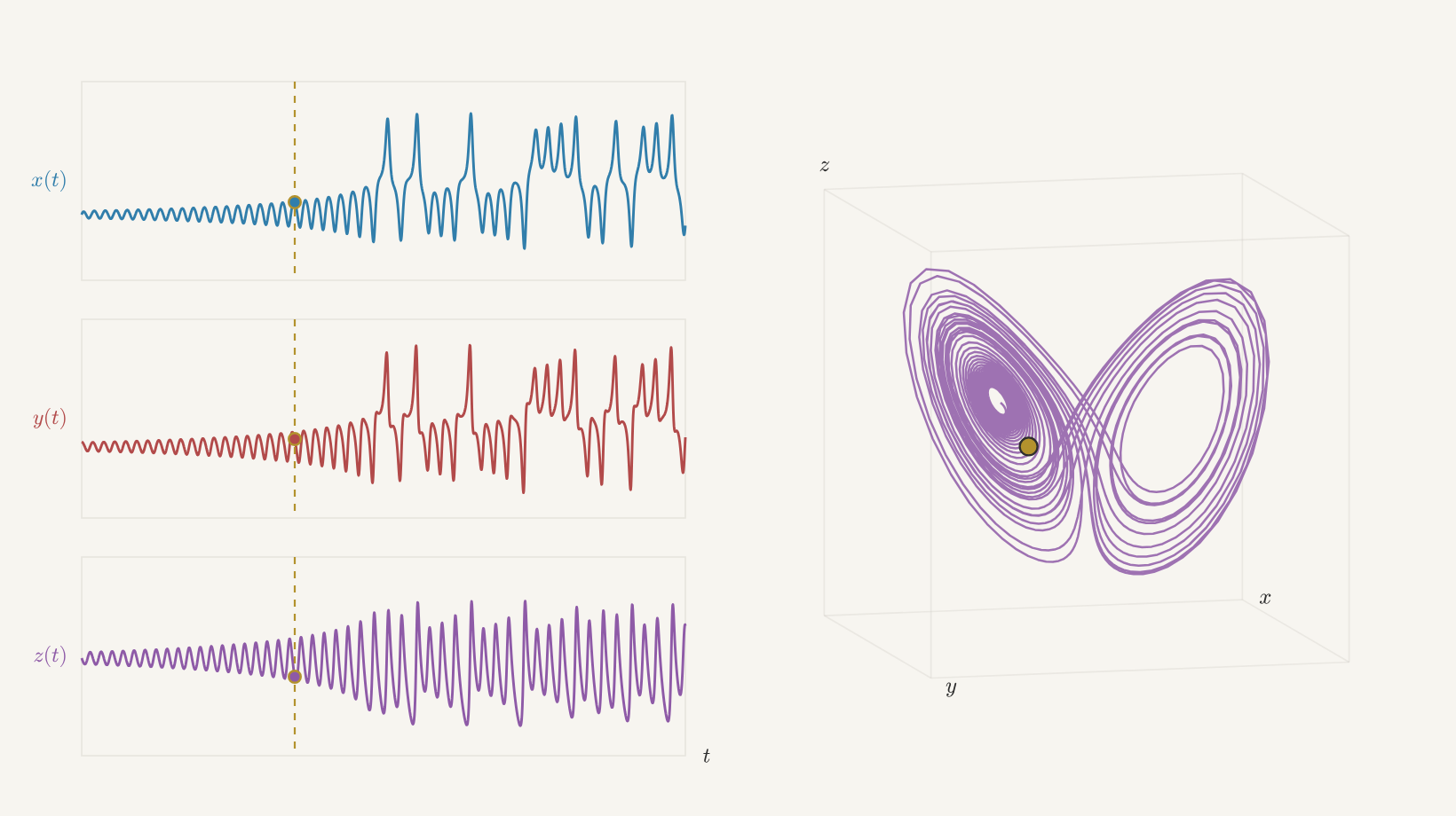
We have learned several ways to picture a solution. But how do we find the functions whose graphs we are drawing? In the next chapter we will put our calculus techniques to work, beginning with the simplest possibility: guess a function and check whether it works.

Problems

The first group checks the language and basic moves of the chapter. The explorations ask you to push those ideas somewhere the text has not already gone. The Python problems begin with supplied code: your job is to read it, change it, and explain the resulting picture.

Check Your Understanding

1Reading a local rule

A room is kept at $20 \circ C$ . An object's temperature satisfies

𝑇' = - 𝑘 (𝑇 - 20), 𝑘 > 0 .

(a)

Is the object warming or cooling when its temperature is $10 \circ C$ ? What about $30 \circ C$ ? At what temperature does the rule prescribe no change?

(b)

Compare the rates of change at $30 \circ C$ and $40 \circ C$ . What does the equation say about their relative sizes?

(c)

Two objects obey this same equation with the same $𝑘$ . One has just been placed in the room; the other has been there for an hour. If both are currently at $30 \circ C$ , what does the rule say about their current rates of change? Does it need to know how they reached that temperature?

2Obeying the equation at a point

Consider the differential equation $𝑦' = 𝑦 2$ .

(a)

Verify by substitution that $𝑦 (𝑡) = 1 2 - 𝑡$ is a solution, on the interval $𝑡 < 2$ .

(b)

The function $𝑧 (𝑡) = 1 1 + 𝑡 2$ is smooth on the whole line, and its graph looks perfectly plausible. Show that it obeys the differential equation at exactly one point, and find that point. (In the language of figure 1.3: this curve is an impostor, and the failure has a location — in fact, every location but one.)

3Checking the equation and the initial condition

Consider

𝑦' = 𝑦, 𝑦 (0) = 2 .

(a)

Check each proposed function against both requirements:

𝑦 (𝑡) = 𝑒 𝑡, 𝑦 (𝑡) = 2 𝑒 𝑡, 𝑦 (𝑡) = 2 + 𝑡 .

Which satisfy the differential equation? Which satisfy the initial condition? Which satisfy both?

(b)

Two proposed solution curves pass through the same point. One has slope $0$ there and the other has slope $1$ . Could both solve the same equation $𝑦' = 𝐹 (𝑡, 𝑦)$ ? Explain using the slope assigned at that point.

(c)

The curves $𝑦 = 0$ and $𝑦 = 𝑡 3$ meet at the origin. Find their slopes there. Does the observation that an equation assigns only one slope at each point rule out both curves being solutions? Explain what that observation does—and does not—tell us.

4A solution you can spot

Suppose all you know about a differential equation is its shape, $𝑦' = (𝑦 - 2 𝑡) 𝑔 (𝑡, 𝑦) + 2$ , where $𝑔$ is some continuous function nobody has told you.

(a)

Show that $𝑦 (𝑡) = 2 𝑡$ is a solution no matter what $𝑔$ is.

(b)

Explain in a sentence why no computation involving $𝑔$ was ever needed.

5Two fields by hand

(a)

On the window $- 2 \leq 𝑡 \leq 2$ , $- 2 \leq 𝑦 \leq 2$ , sketch the slope field of $𝑦' = - 𝑦$ by hand, evaluating at integer points. Then do the same for $𝑦' = 𝑡$ on a second copy of the window.

(b)

Each of your two fields repeats itself, but in different directions: one is unchanged as you slide the picture horizontally, the other as you slide it vertically. Say which is which, and explain how you could have predicted this from the equations without drawing anything.

(c)

On each sketch, draw the solution curve passing through $(0, 1)$ by following your ticks.

6Three rules, three signatures

Consider the three equations $𝑦' = 1 - 𝑡$ , $𝑦' = 𝑡 - 2 𝑦$ , and $𝑦' = 𝑡 (1 - 𝑦)$ . For each equation, find all points where the prescribed slope is zero, and sketch the resulting lines. Then decide whether its field repeats along vertical lines, horizontal lines, or neither. Explain how these signatures would let you recognize the equation from its slope field without solving it.

Explorations

7The shape of the field is the shape of the rule

(a)

A slope field has the property that its ticks are identical along every vertical line. What does this say about the right-hand side $𝐹 (𝑡, 𝑦)$ ?

(b)

Another field has ticks identical along every horizontal line. What does this say about $𝐹$ ?

(c)

For an equation of the kind in the previous part — one whose rule involves only $𝑦$ , say $𝑦' = 𝑓 (𝑦)$ — show that sliding a solution in time produces another solution: if $𝑦 (𝑡)$ is a solution and $𝑐$ is any constant, then $𝑧 (𝑡) = 𝑦 (𝑡 - 𝑐)$ is also a solution. Explain how this fact and the horizontal repetition of the field are the same observation made twice.

8One curve, two shadows

Consider the system $𝑓' = 𝑔$ , $𝑔' = - 𝑓$ .

(a)

Verify that $𝑓 (𝑡) = s i n 𝑡$ and $𝑔 (𝑡) = c o s 𝑡$ solve both equations.

(b)

Write the direction assigned by the system at $(𝑡, 𝑓, 𝑔) = (0, 2, - 3)$ . Interpret the signs of its three components.

(c)

Draw the graphs of $𝑓 (𝑡)$ and $𝑔 (𝑡)$ in separate panels with the same time scale. Use $𝑓' = 𝑔$ and $𝑔' = - 𝑓$ to explain how the height of either graph determines the slope of the other at the same time.

Python: Plotting Local Rules

These problems use NumPy and Matplotlib. Begin with the supplied code and make one change at a time; a plot is part of your answer, but so is the sentence which explains what it shows.

9Build a slope field

The code below draws the slope field of $𝑦' = 𝑡 - 𝑦$ .

import numpy as np
import matplotlib.pyplot as plt

t = np.linspace(-3, 3, 21)
y = np.linspace(-3, 3, 21)
T, Y = np.meshgrid(t, y)
S = T - Y

length = np.sqrt(1 + S**2)
plt.quiver(T, Y, 1 / length, S / length,
           angles="xy", pivot="mid", color="steelblue")
plt.xlabel("t")
plt.ylabel("y")
plt.show()

(a)

Explain the jobs of meshgrid, S, and length. Why do the two components passed to quiver describe a segment of slope $𝑆$ ?

(b)

Change only the line defining S to draw the fields of $𝑦' = - 𝑦$ and $𝑦' = 𝑡$ . For each field, identify the direction in which the pattern repeats.

(c)

Create a Boolean mask for points where abs(S) < 0.15 and plot those points on top of one field. What curve is your code detecting?

10Plot the components of a solution

Use the following samples from the solution of $𝑓' = 𝑔$ , $𝑔' = - 𝑓$ .

t = np.linspace(0, 4 * np.pi, 500)
f = np.sin(t)
g = np.cos(t)

Create a figure with two panels: $𝑓$ against $𝑡$ and $𝑔$ against $𝑡$ . Give every axis a label and use the same time scale in both panels. Mark the two values at $𝑡 = 𝜋 / 4$ . Explain why the two graphs together describe one solution of the system, and why either graph alone does not show its full slope field.