Forcing and Linear Response

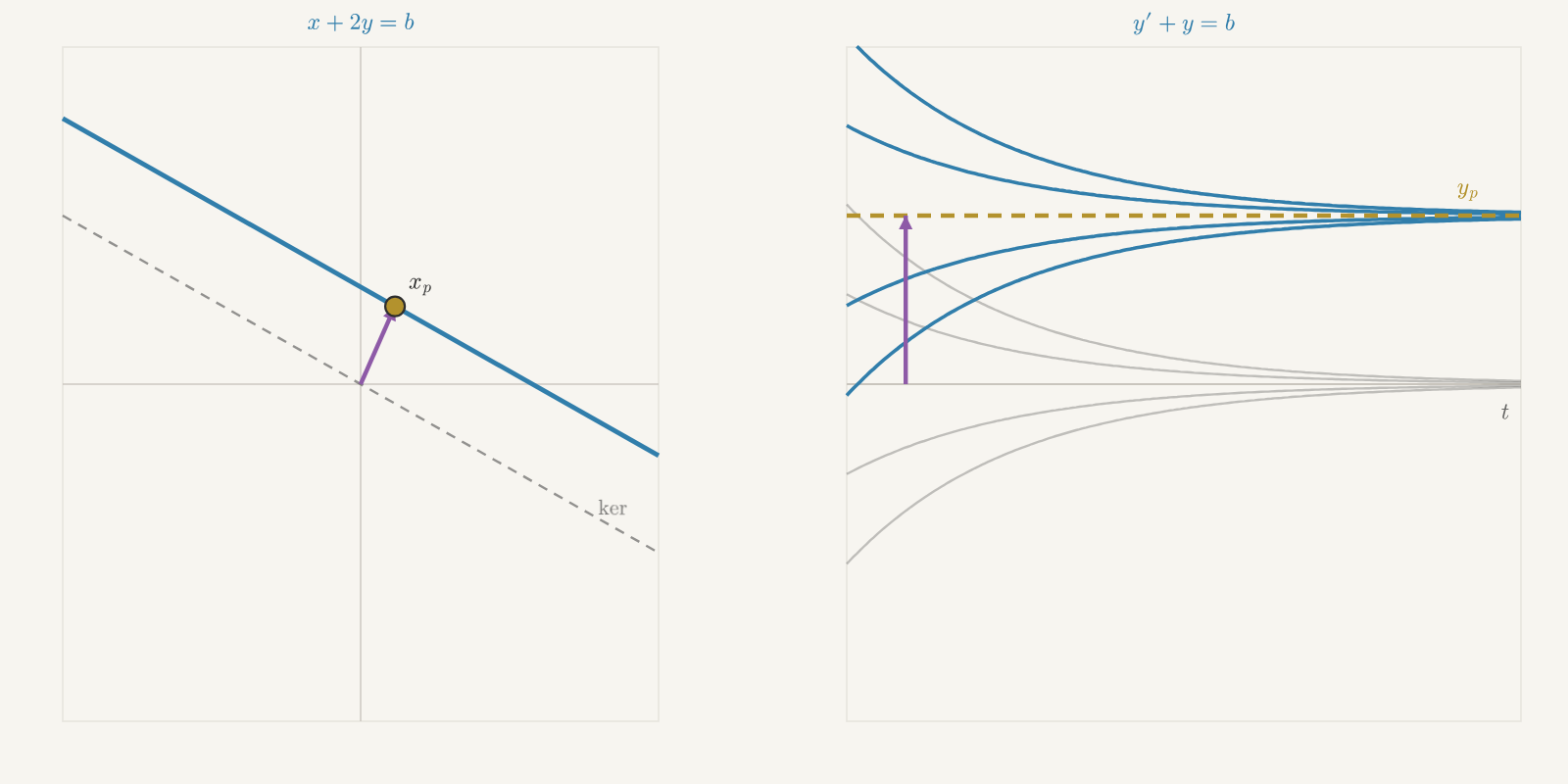
Open with Newton cooling supplied by a constant heater. The input shifts the equilibrium, while every solution differs from that equilibrium by a homogeneous cooling history.

Compare the result with 𝐴𝐱 =𝐛: one particular solution plus a solution of 𝐴𝐱 =0. For differential equations, prove that two solutions with the same forcing differ by a homogeneous solution, and conclude that every solution is one particular solution plus a homogeneous solution.

Describe the forced solution family as an affine translate of the homogeneous solution space. Keep the language of null spaces, bases, and translates from ordinary linear algebra without introducing a differential operator or its kernel.

Use this affine description as the starting point for constructing responses to time-dependent forcing later in the chapter.

Build the greenhouse-air and rock-bed model 𝑈′ =𝐾𝑈 +𝑏 from heat exchange. Find its equilibrium 𝑈∗ and shift to the deviation 𝑉 =𝑈 −𝑈∗, which satisfies the homogeneous system 𝑉′ =𝐾𝑉.

Use the already-developed homogeneous flow to write 𝑈(𝑡) =𝑈∗ +Φ(𝑡)(𝑈0 −𝑈∗). Interpret this as an equilibrium plus a freely evolving deviation.

Keep the application focused on the relationship between forced and free response. Do not repeat the construction of the flow matrix or the earlier development of eigenvalues, eigenvectors, and modes.

Retain connected mixing tanks as a possible substantial problem: derive the forced system, find its equilibrium, subtract it, and reuse its homogeneous flow.

Use the equilibrium shift as a simple entry into the chapter's larger question: how does a linear system transform a changing external input into an observable response?