Chapter 7

The Matrix Exponential

Chapter 6 left us with a matrix initial value problem. For the system $𝑋' = 𝐴 (𝑡) 𝑋$ , the flow matrix beginning at time $𝑡 0$ satisfies

Φ' 𝑡 0 (𝑡) = 𝐴 (𝑡) Φ 𝑡 0 (𝑡), Φ 𝑡 0 (𝑡 0) = 𝐼 .

We can construct this matrix by solving once from each standard initial state, either exactly or numerically. That procedure computes the columns of $Φ 𝑡 0$ separately. It does not yet tell us how to construct the whole matrix directly from the coefficient matrix $𝐴 (𝑡)$ .

We now restrict attention to a constant system $𝑋' = 𝐴 𝑋$ . In this case the starting time can be removed by resetting the clock. If $𝑋 (𝑡 0) = 𝑋 0$ , define $𝑌 (𝜏) = 𝑋 (𝑡 0 + 𝜏)$ . The chain rule gives

𝑌' (𝜏) = 𝑋' (𝑡 0 + 𝜏) = 𝐴 𝑋 (𝑡 0 + 𝜏) = 𝐴 𝑌 (𝜏), 𝑌 (0) = 𝑋 0 .

Thus the evolution depends only on the elapsed time $𝜏 = 𝑡 - 𝑡 0$ : $Φ 𝑡 0 (𝑡) = Φ 0 (𝑡 - 𝑡 0)$ . We may set the initial time equal to zero, construct $Φ 0 (𝑡)$ , and replace $𝑡$ by $𝑡 - 𝑡 0$ when the original clock is needed.

The problem is therefore precise: given a constant $𝑁 \times 𝑁$ matrix $𝐴$ , construct the matrix-valued solution of

Φ' (𝑡) = 𝐴 Φ (𝑡), Φ (0) = 𝐼

directly from $𝐴$ .

7.1The Generator of Rotation

The solutions of the normalized spring $𝑥 ″ = - 𝑥$ are already known. With state $𝑋 = (𝑥, 𝑣)$ , where $𝑣 = 𝑥'$ , its equation becomes the constant system

𝑋' = (𝑥' 𝑣') = (𝑣 - 𝑥) = (01 - 1 0) (𝑥 𝑣) = 𝐽 𝑋, 𝐽 = (01 - 1 0) .

At a state $𝑋 = (𝑥, 𝑣)$ , the matrix $𝐽$ assigns the velocity $𝐽 𝑋 = (𝑣, - 𝑥)$ . This vector is perpendicular to $𝑋$ , since $(𝑥, 𝑣) \cdot (𝑣, - 𝑥) = 𝑥 𝑣 - 𝑣 𝑥 = 0$ , and it has the same length because $‖ 𝐽 𝑋 ‖ 2 = 𝑣 2 + 𝑥 2 = ‖ 𝑋 ‖ 2$ . Thus the differential equation prescribes clockwise motion tangent to the circle through the current state, with unit angular speed.

We also know the solution from an arbitrary initial state $𝑋 0 = (𝑥 0, 𝑣 0)$ . The position and velocity are

𝑥 (𝑡) = 𝑥 0 c o s 𝑡 + 𝑣 0 s i n 𝑡, 𝑣 (𝑡) = - 𝑥 0 s i n 𝑡 + 𝑣 0 c o s 𝑡 .

Putting these two equations into a single matrix equation gives

𝑋 (𝑡) = 𝑅 (𝑡) 𝑋 0, 𝑅 (𝑡) = (c o s 𝑡 s i n 𝑡 - s i n 𝑡 c o s 𝑡) .

The matrix $𝐽$ describes the velocity at one instant, while $𝑅 (𝑡)$ advances every initial state through a time interval of length $𝑡$ . These matrices are connected by the same equation that governed the flow matrix in Chapter 6. Indeed,

𝑅' (𝑡) = (- s i n 𝑡 c o s 𝑡 - c o s 𝑡 - s i n 𝑡), 𝐽 𝑅 (𝑡) = (01 - 1 0) (c o s 𝑡 s i n 𝑡 - s i n 𝑡 c o s 𝑡) = (- s i n 𝑡 c o s 𝑡 - c o s 𝑡 - s i n 𝑡) .

Therefore $𝑅' (𝑡) = 𝐽 𝑅 (𝑡)$ , and direct evaluation gives $𝑅 (0) = 𝐼$ . In particular,

𝑅' (0) = 𝐽 𝑅 (0) = 𝐽 .

Here we obtained $𝑅 (𝑡)$ from a solution formula that was already available. If the sine and cosine formulas were not known, how could we recover $𝑅 (𝑡)$ from the matrix $𝐽$ alone?

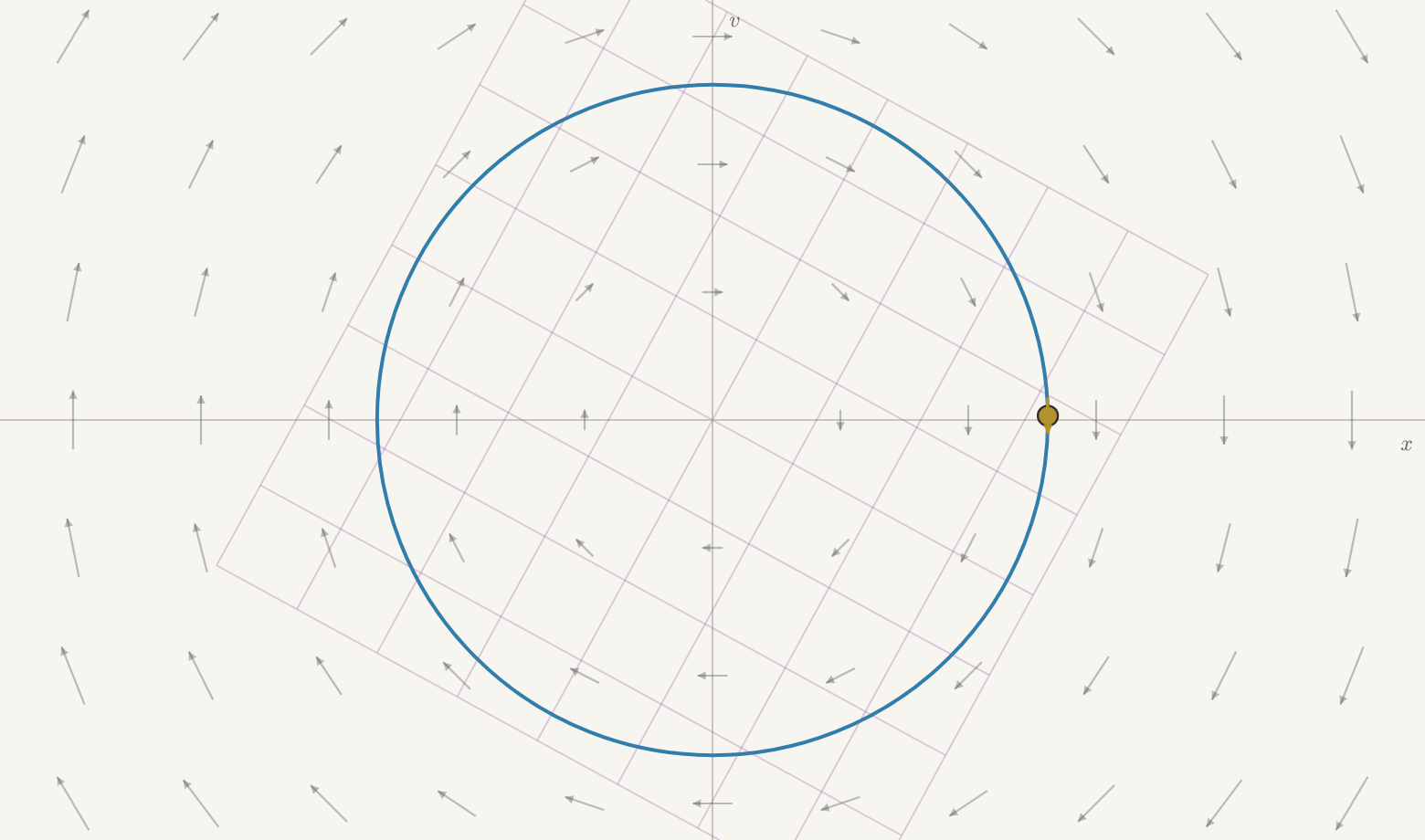
Figure 7.1 For $𝑋' = 𝐽 𝑋$ , every velocity arrow is perpendicular to the position vector and grows in proportion to its length. The state therefore travels around a circle while the grid rotates rigidly with it. In the live figure, drag the gold state and watch the entries of the rotation matrix $𝑅 (𝑡)$ change as the motion continues.

7.2Repeated Small Steps

Before trying to recover the rotation matrix from $𝐽$ , consider the scalar equation with the same constant-coefficient form:

𝑦' = 𝑎 𝑦, 𝑦 (0) = 𝑦 0 .

Euler's method with step size $ℎ$ replaces the continuous evolution by the repeated update

𝑦 𝑘 + 1 = 𝑦 𝑘 + ℎ 𝑎 𝑦 𝑘 = (1 + ℎ 𝑎) 𝑦 𝑘 .

To travel from time $0$ to time $𝑡$ in $𝑛$ equal steps, take $ℎ = 𝑡 / 𝑛$ . Repeating the update $𝑛$ times gives

𝑦 𝑛 = (1 + 𝑎 𝑡 𝑛) 𝑛 𝑦 0 .

Calculus identifies the limit of these growth factors:

𝑒 𝑎 𝑡 = l i m 𝑛 \to \infty (1 + 𝑎 𝑡 𝑛) 𝑛 .

Now apply exactly the same numerical idea to $𝑋' = 𝐴 𝑋$ . One Euler step sends the current state $𝑋 𝑘$ to

𝑋 𝑘 + 1 = 𝑋 𝑘 + ℎ 𝐴 𝑋 𝑘 = (𝐼 + ℎ 𝐴) 𝑋 𝑘 .

Because $𝐴$ is constant, every step uses the same matrix. After $𝑛$ steps of size $𝑡 / 𝑛$ , the computed state is therefore

𝑋 𝑛 = (𝐼 + 𝑡 𝑛 𝐴) 𝑛 𝑋 0 .

For the spring generator $𝐽$ , we can see precisely what these repeated updates do. The preceding section showed that $𝐽 𝑋$ is perpendicular to $𝑋$ and has the same length. Thus the new radius $𝑋 + ℎ 𝐽 𝑋$ is the hypotenuse of a right triangle whose perpendicular legs are $𝑋$ and $ℎ 𝐽 𝑋$ . The Pythagorean theorem gives

‖ 𝑋 + ℎ 𝐽 𝑋 ‖ 2 = ‖ 𝑋 ‖ 2 + ℎ 2 ‖ 𝐽 𝑋 ‖ 2 = (1 + ℎ 2) ‖ 𝑋 ‖ 2 .

One step therefore multiplies every length by $\sqrt 1 + ℎ 2$ . Its signed clockwise turning angle is $a r c t a n ℎ$ : the ratio of the perpendicular leg to the original radius is $ℎ$ . In terms of the rotation matrix from the previous section, the entire Euler update is

𝐼 + ℎ 𝐽 = \sqrt 1 + ℎ 2 𝑅 (a r c t a n ℎ) .

Repeating this same scaling and rotation $𝑛$ times, with $ℎ = 𝑡 / 𝑛$ , yields

(𝐼 + 𝑡 𝑛 𝐽) 𝑛 = (1 + 𝑡 2 𝑛 2) 𝑛 / 2 𝑅 (𝑛 a r c t a n 𝑡 𝑛) .

Both finite-step errors are visible here. The first factor makes the state spiral outward, while the angle after $𝑛$ steps is not quite $𝑡$ . But both errors disappear as the step size shrinks. For the radial factor,

0 \leq 𝑛 2 l o g (1 + 𝑡 2 𝑛 2) \leq 𝑡 2 2 𝑛 ⟶ 0,

so $(1 + 𝑡 2 / 𝑛 2) 𝑛 / 2 \to 1$ . When $𝑡 \neq 0$ , the accumulated angle satisfies

𝑛 a r c t a n 𝑡 𝑛 = 𝑡 a r c t a n (𝑡 / 𝑛) 𝑡 / 𝑛 ⟶ 𝑡,

and the case $𝑡 = 0$ is immediate. Consequently,

(𝐼 + 𝑡 𝑛 𝐽) 𝑛 ⟶ 𝑅 (𝑡) .

Starting only from the local rule $𝐽$ , Euler's small linear turns recover the exact rotation in the limit.

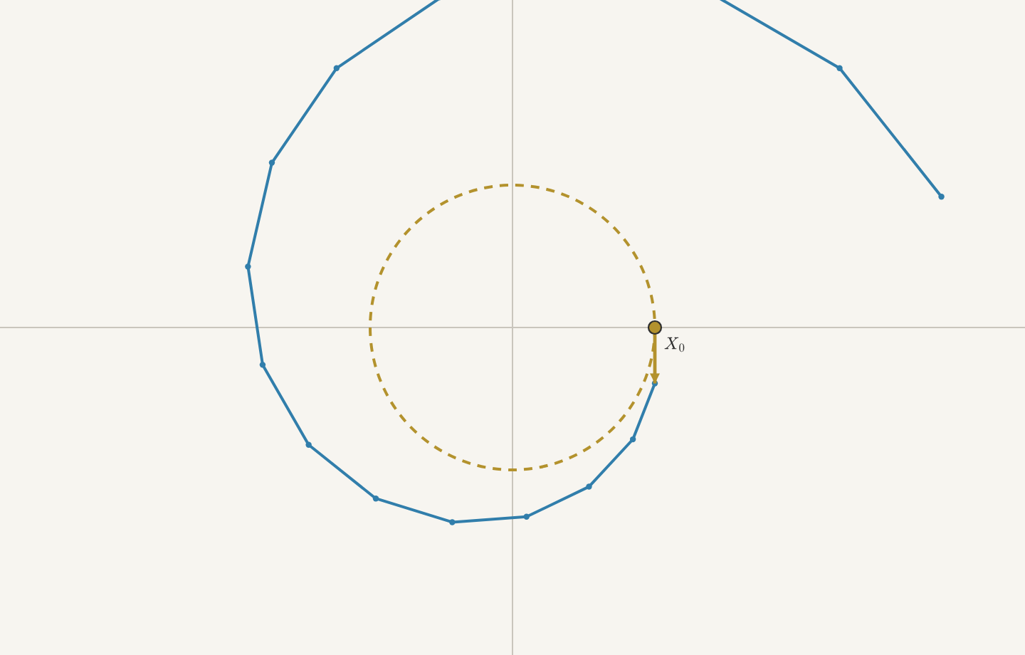
Figure 7.2 Each Euler step multiplies the state by $𝐼 + ℎ 𝐽$ . This turns the state through $a r c t a n ℎ$ , but it also stretches lengths by $\sqrt 1 + ℎ 2$ , so the polygon spirals outside the true circle. In the live figure, increase the number of steps per loop: the accumulated stretch shrinks and $(𝐼 + 𝑡 𝑛 𝐽) 𝑛$ approaches the rotation $𝑅 (𝑡)$ .

The scalar and matrix calculations now have the same shape:

𝑒 𝑎 𝑡 = l i m 𝑛 \to \infty (1 + 𝑎 𝑡 𝑛) 𝑛, 𝑅 (𝑡) = l i m 𝑛 \to \infty (𝐼 + 𝑡 𝑛 𝐽) 𝑛 .

For a general constant matrix $𝐴$ , this resemblance suggests both a name and a possible limiting formula for the exact flow:

𝑒 𝑡 𝐴 ? = l i m 𝑛 \to \infty (𝐼 + 𝑡 𝑛 𝐴) 𝑛 .

The question mark matters. We have proved this matrix limit only for the special generator $𝐽$ , and an Euler approximation does not by itself define the exact solution. The exact equation $Φ' = 𝐴 Φ$ , $Φ (0) = 𝐼$ must tell us what the matrix $𝑒 𝑡 𝐴$ is.

7.3The Matrix Exponential

The Euler product suggested what to call the flow, but the exact equation must construct it. We return to

Φ' = 𝐴 Φ, Φ (0) = 𝐼 .

For the scalar equation $𝑦' = 𝑎 𝑦$ , the initial condition $𝑦 (0) = 1$ characterizes $𝑒 𝑎 𝑡$ . The matrix equation has precisely the same form: the scalar $1$ has become the identity matrix $𝐼$ , and multiplication by the number $𝑎$ has become left multiplication by the matrix $𝐴$ . If a matrix-valued function deserves to be called $𝑒 𝑡 𝐴$ , it is the solution of this initial value problem.

There is nothing mysterious about differentiating such a function. The set $𝑀 𝑁 (ℝ)$ of real $𝑁 \times 𝑁$ matrices is a vector space with $𝑁 2$ coordinates, one for each entry. A matrix-valued function is a curve in this space, and its derivative is computed entry by entry. Moreover, the map $𝐵 \mapsto 𝐴 𝐵$ is linear on $𝑀 𝑁 (ℝ)$ . Thus the equation above is an ordinary linear system in $𝑁 2$ scalar coordinates. Viewed column by column, it is also exactly the collection of $𝑁$ standard-history problems from Chapter 6.

How might we construct its solution? In Calculus II, power series gave a way to solve differential equations when no formula was yet available. Try the same idea here by seeking a candidate of the form

Φ (𝑡) = 𝐶 0 + 𝐶 1 𝑡 + 𝐶 2 𝑡 2 + 𝐶 3 𝑡 3 + \dots,

where each coefficient $𝐶 𝑘$ is a constant matrix. We are not assuming that an unknown solution must be analytic; we are asking whether a power series can produce one. Formally differentiating the candidate and multiplying it by $𝐴$ give

Φ' (𝑡) = 𝐶 1 + 2 𝐶 2 𝑡 + 3 𝐶 3 𝑡 2 + \dots, 𝐴 Φ (𝑡) = 𝐴 𝐶 0 + 𝐴 𝐶 1 𝑡 + 𝐴 𝐶 2 𝑡 2 + \dots .

The initial condition requires $𝐶 0 = 𝐼$ . Matching equal powers of $𝑡$ in the differential equation then requires

𝐶 1 = 𝐴 𝐶 0 = 𝐴, 2 𝐶 2 = 𝐴 𝐶 1 = 𝐴 2, 3 𝐶 3 = 𝐴 𝐶 2 = 𝐴 3 2! .

In general, $(𝑘 + 1) 𝐶 𝑘 + 1 = 𝐴 𝐶 𝑘$ , so the pattern continues by induction:

𝐶 𝑘 = 𝐴 𝑘 𝑘! .

We have therefore arrived at one possible solution,

𝐼 + 𝑡 𝐴 + 𝑡 2 𝐴 2 2! + 𝑡 3 𝐴 3 3! + \dots .

So far this is only a formal candidate. Before differentiating it as though it were a function, we must know that its partial sums actually converge. For a matrix $𝐵 = (𝑏 𝑖 𝑗)$ , define the row-sum norm

‖ 𝐵 ‖ = m a x 𝑖 \sum 𝑗 | 𝑏 𝑖 𝑗 | .

This is also commonly called the infinity norm, though we will use the more descriptive name here.

This norm interacts especially well with matrix multiplication. If $𝐵 = (𝑏 𝑖 𝑗)$ and $𝐶 = (𝑐 𝑖 𝑗)$ , then

‖ 𝐵 𝐶 ‖ = m a x 𝑖 \sum 𝑗 ∣ \sum ℓ 𝑏 𝑖 ℓ 𝑐 ℓ 𝑗 ∣ \leq m a x 𝑖 \sum ℓ | 𝑏 𝑖 ℓ | \sum 𝑗 | 𝑐 ℓ 𝑗 | \leq (m a x 𝑖 \sum ℓ | 𝑏 𝑖 ℓ |) (m a x ℓ \sum 𝑗 | 𝑐 ℓ 𝑗 |) = ‖ 𝐵 ‖ ‖ 𝐶 ‖ .

Applying this inequality repeatedly gives $‖ 𝐴 𝑘 ‖ \leq ‖ 𝐴 ‖ 𝑘$ . Consequently,

∥ 𝑡 𝑘 𝐴 𝑘 𝑘! ∥ \leq | 𝑡 | 𝑘 ‖ 𝐴 ‖ 𝑘 𝑘! .

The scalar series formed from the quantities on the right is

\infty \sum 𝑘 = 0 | 𝑡 | 𝑘 ‖ 𝐴 ‖ 𝑘 𝑘! = 𝑒 | 𝑡 | ‖ 𝐴 ‖,

which converges for every real $𝑡$ . The comparison therefore proves that our matrix series converges for every $𝑡$ as well. Since $𝑀 𝑁 (ℝ)$ has only finitely many coordinates, convergence in this norm is equivalent to convergence of every matrix entry.

We may now make the promised definition.

Definition 7.1 (Matrix exponential). For a real square matrix $𝐴$ , its matrix exponential is the matrix-valued function

𝑒 𝑡 𝐴 : = \infty \sum 𝑘 = 0 𝑡 𝑘 𝐴 𝑘 𝑘! .

The notation does not mean that we exponentiate the entries of $𝐴$ separately. It names the matrix built from the powers $𝐼, 𝐴, 𝐴 2, 𝐴 3, \dots$ by this convergent series.

Each entry of the matrix exponential is now a scalar power series with infinite radius of convergence. The power-series theorem from calculus therefore permits term-by-term differentiation. Reindexing the resulting series gives

𝑑 𝑑 𝑡 𝑒 𝑡 𝐴 = \infty \sum 𝑘 = 1 𝑘 𝑡 𝑘 - 1 𝐴 𝑘 𝑘! = 𝐴 \infty \sum 𝑘 = 1 𝑡 𝑘 - 1 𝐴 𝑘 - 1 (𝑘 - 1)! = 𝐴 𝑒 𝑡 𝐴 .

At $𝑡 = 0$ , every term except the first vanishes, so $𝑒 0 𝐴 = 𝐼$ . The series really does solve the matrix initial value problem that produced it. Uniqueness now identifies it with the flow matrix.

Theorem 7.2 (Flow of a constant linear system). For a constant real matrix $𝐴$ , the unique solution of

𝑋' = 𝐴 𝑋, 𝑋 (𝑡 0) = 𝑋 0

𝑋 (𝑡) = 𝑒 (𝑡 - 𝑡 0) 𝐴 𝑋 0 .

Proof. Set $𝑋 (𝑡) = 𝑒 (𝑡 - 𝑡 0) 𝐴 𝑋 0$ . The calculation above gives

𝑋' (𝑡) = 𝐴 𝑒 (𝑡 - 𝑡 0) 𝐴 𝑋 0 = 𝐴 𝑋 (𝑡),

while $𝑋 (𝑡 0) = 𝑒 0 𝐴 𝑋 0 = 𝑋 0$ . Thus this function satisfies both the differential equation and the initial condition. Uniqueness says it is the solution. ∎

The spring shows what this construction has accomplished. Since $𝐽 2 = - 𝐼$ , the powers repeat in groups of four: $𝐽 3 = - 𝐽$ and $𝐽 4 = 𝐼$ . Because the exponential series converges absolutely, we may collect its even and odd powers to obtain

𝑒 𝑡 𝐽 = 𝐼 + 𝑡 𝐽 + 𝑡 2 𝐽 2 2! + 𝑡 3 𝐽 3 3! + \dots = 𝐼 (1 - 𝑡 2 2! + 𝑡 4 4! - \dots) + 𝐽 (𝑡 - 𝑡 3 3! + 𝑡 5 5! - \dots) = 𝐼 c o s 𝑡 + 𝐽 s i n 𝑡 = 𝑅 (𝑡) .

We began with the instantaneous rule $𝐽$ and, without assuming the trigonometric solution, constructed the entire rotation flow from its powers.

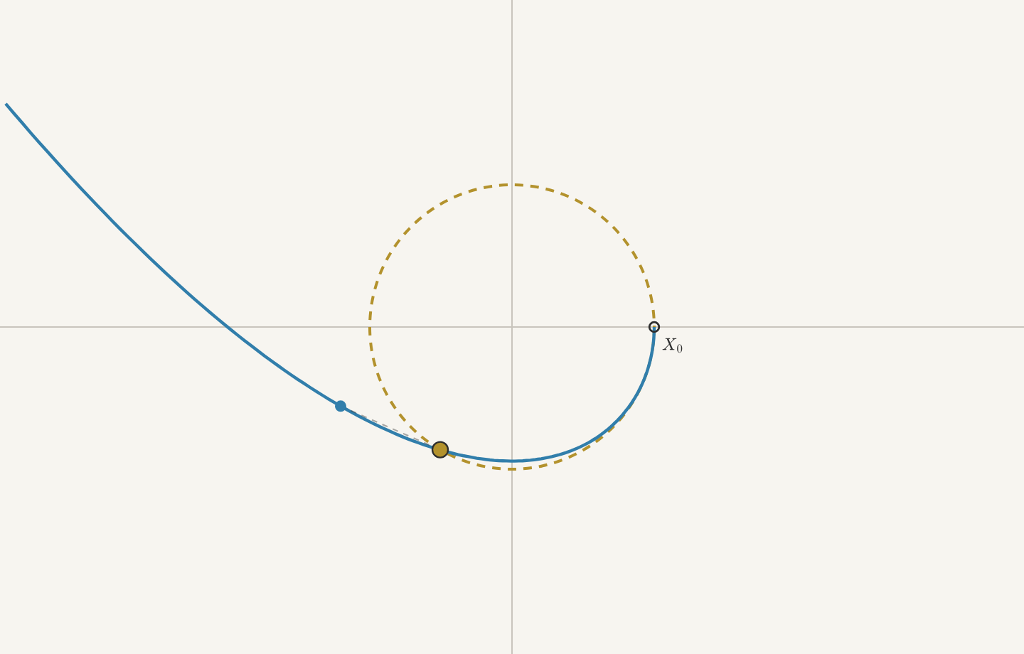
Figure 7.3 In the live figure, choose how many terms of the exponential series to keep. The resulting polynomial path follows the true circle for longer as more terms are added, then eventually peels away. Drag the gold state around the circle to compare its true position with the position predicted by the chosen truncation. In the limit, the series produces the flow we denote by $𝑒 𝑡 𝐽$ .

The matrix exponential also obeys the familiar law for adding elapsed times. Fix $𝑠$ and consider, as functions of $𝑡$ ,

𝐹 (𝑡) = 𝑒 (𝑡 + 𝑠) 𝐴, 𝐺 (𝑡) = 𝑒 𝑡 𝐴 𝑒 𝑠 𝐴 .

Both satisfy $𝑍' = 𝐴 𝑍$ , and both equal $𝑒 𝑠 𝐴$ when $𝑡 = 0$ . Uniqueness gives

𝑒 (𝑡 + 𝑠) 𝐴 = 𝑒 𝑡 𝐴 𝑒 𝑠 𝐴 .

Taking $𝑠 = - 𝑡$ then gives

𝑒 𝑡 𝐴 𝑒 - 𝑡 𝐴 = 𝑒 0 𝐴 = 𝐼, (𝑒 𝑡 𝐴) - 1 = 𝑒 - 𝑡 𝐴 .

Thus every constant linear system produces an invertible flow for every elapsed time. The remaining difficulty is computational: when the powers of $𝐴$ do not repeat as transparently as the powers of $𝐽$ , how can we recognize the motion encoded by their series?

7.4Matrix Flows We Can Compute

The exponential series gives an exact flow for every constant matrix, but an infinite series is not always the most revealing form of the answer. For some matrices, the pattern in the powers turns the series into a familiar formula and makes the resulting motion visible.

Begin with a scalar multiple of the identity, $𝐴 = 𝜆 𝐼$ . Since $(𝜆 𝐼) 𝑘 = 𝜆 𝑘 𝐼$ , every term of the matrix series is a scalar multiple of the identity:

𝑒 𝑡 𝐴 = \infty \sum 𝑘 = 0 𝑡 𝑘 (𝜆 𝐼) 𝑘 𝑘! = (\infty \sum 𝑘 = 0 (𝜆 𝑡) 𝑘 𝑘!) 𝐼 = 𝑒 𝜆 𝑡 𝐼 .

The local rule $𝐴 𝑋 = 𝜆 𝑋$ points along the line through $𝑋$ , outward when $𝜆 > 0$ and inward when $𝜆 < 0$ . Its flow multiplies every state by the same factor $𝑒 𝜆 𝑡$ , so every state remains on its original ray.

The coordinates can also grow at different rates. If

𝐷 = (𝜆 1 0 0 𝜆 2),

then every power of $𝐷$ is still diagonal:

𝐷 𝑘 = (𝜆 𝑘 1 0 0 𝜆 𝑘 2) .

Substitution into the series gives

𝑒 𝑡 𝐷 = (𝑒 𝜆 1 𝑡 0 0 𝑒 𝜆 2 𝑡),

and therefore

𝑒 𝑡 𝐷 (𝑥 0 𝑦 0) = (𝑒 𝜆 1 𝑡 𝑥 0 𝑒 𝜆 2 𝑡 𝑦 0) .

This formula may look like entrywise exponentiation, but it works only because the diagonal matrix does not mix the coordinates. The two scalar equations $𝑥' = 𝜆 1 𝑥$ and $𝑦' = 𝜆 2 𝑦$ evolve independently. In particular, $𝐷 = d i a g (1, - 1)$ expands the first coordinate while contracting the second as time moves forward.

Some matrices simplify for a different reason: their higher powers vanish. Consider

𝑁 = (0100) .

Here $𝑁 2 = 0$ , so every term of the exponential series after the linear term vanishes:

𝑒 𝑡 𝑁 = 𝐼 + 𝑡 𝑁 = (1 𝑡 01) .

Thus the flow sends

(𝑥 0, 𝑦 0) ⟼ (𝑥 0 + 𝑡 𝑦 0, 𝑦 0) .

The second coordinate remains fixed while the first changes at the constant rate $𝑦 0$ . Every point on the $𝑥$ -axis is fixed, and horizontal layers slide past one another faster when they lie farther from that axis. This is a shear.

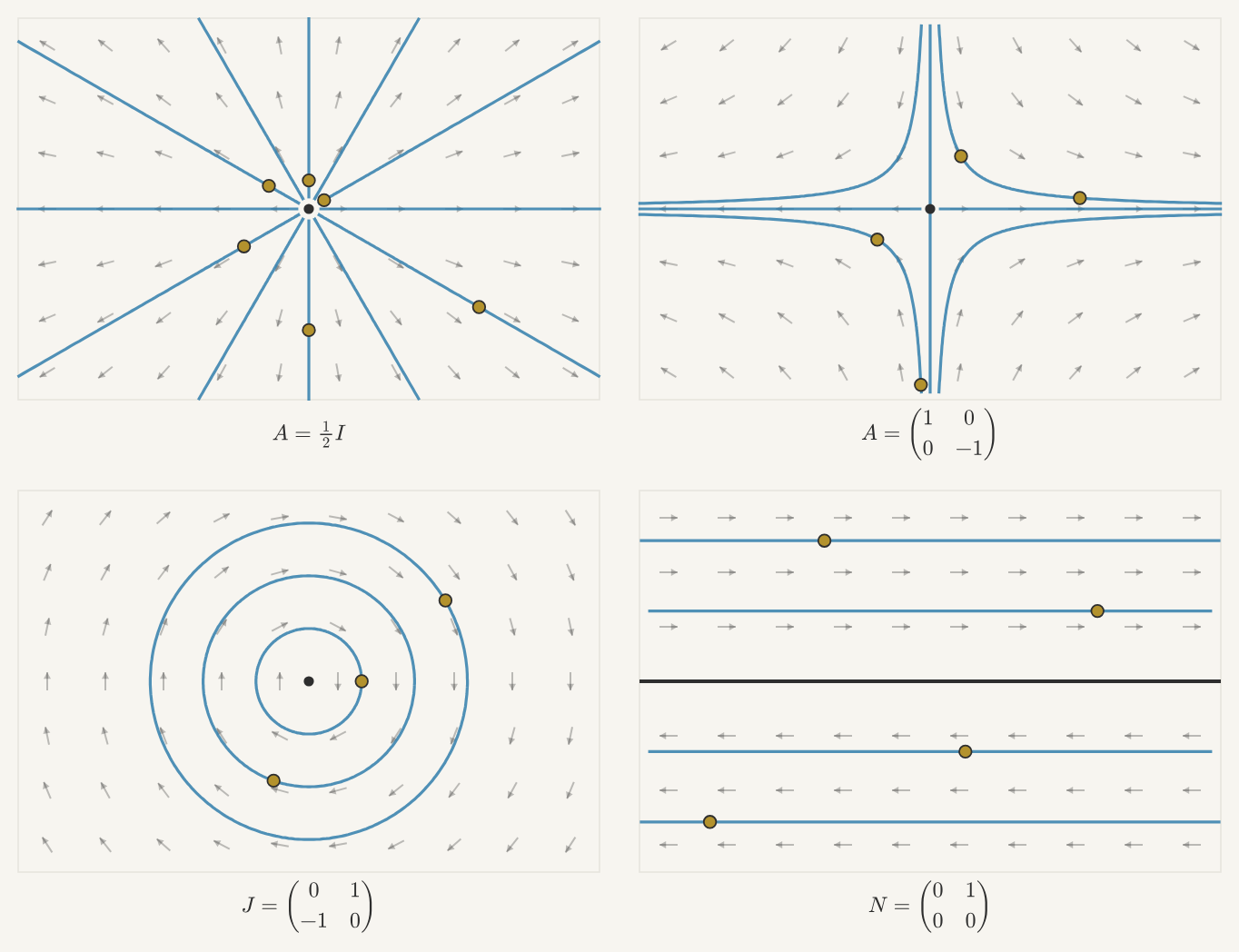
Figure 7.4 These four matrices have simple patterns in their powers but produce quite different motion. Uniform scaling pushes every ray outward, diagonal scaling gives the two axes different rates, $𝐽$ rotates the plane, and the nilpotent matrix slides horizontal layers past one another while leaving the $𝑥$ -axis fixed. The gold states move at the speeds prescribed by their respective vector fields.

The first and third of these motions can occur simultaneously. Suppose

𝐴 = 𝑎 𝐼 + 𝜔 𝐽 .

At each state $𝑋$ , the term $𝑎 𝑋$ points radially while $𝜔 𝐽 𝑋$ points tangentially. This suggests a flow that scales by $𝑒 𝑎 𝑡$ while rotating through the angle $𝜔 𝑡$ . To check that the two motions really combine in this way, set

𝐹 (𝑡) = 𝑒 𝑎 𝑡 (𝐼 c o s (𝜔 𝑡) + 𝐽 s i n (𝜔 𝑡)) .

Using $𝐽 2 = - 𝐼$ , differentiation gives

𝐹' (𝑡) = 𝑒 𝑎 𝑡 (𝑎 𝐼 c o s (𝜔 𝑡) + 𝑎 𝐽 s i n (𝜔 𝑡) - 𝜔 𝐼 s i n (𝜔 𝑡) + 𝜔 𝐽 c o s (𝜔 𝑡)),

while multiplication by $𝐴$ gives

𝐴 𝐹 (𝑡) = 𝑒 𝑎 𝑡 (𝑎 𝐼 + 𝜔 𝐽) (𝐼 c o s (𝜔 𝑡) + 𝐽 s i n (𝜔 𝑡)) = 𝑒 𝑎 𝑡 (𝑎 𝐼 c o s (𝜔 𝑡) + 𝑎 𝐽 s i n (𝜔 𝑡) + 𝜔 𝐽 c o s (𝜔 𝑡) - 𝜔 𝐼 s i n (𝜔 𝑡)) .

The two expressions agree, and $𝐹 (0) = 𝐼$ . Uniqueness therefore proves

𝑒 𝑡 (𝑎 𝐼 + 𝜔 𝐽) = 𝑒 𝑎 𝑡 (𝐼 c o s (𝜔 𝑡) + 𝐽 s i n (𝜔 𝑡)) .

When $𝑎 > 0$ , states spiral outward; when $𝑎 < 0$ , they spiral inward; and when $𝑎 = 0$ , we recover the circular motion of the normalized spring. The magnitude of $𝜔$ sets the angular speed, while its sign sets the direction.

We can also write the formula as

𝑒 𝑡 (𝑎 𝐼 + 𝜔 𝐽) = 𝑒 𝑡 𝑎 𝐼 𝑒 𝑡 𝜔 𝐽 .

This factorization works because $𝑎 𝐼$ and $𝜔 𝐽$ commute. It is not a general law: if two matrices $𝐵$ and $𝐶$ do not commute, then $𝑒 𝐵 + 𝐶$ need not equal $𝑒 𝐵 𝑒 𝐶$ .

These examples succeeded because the powers of each matrix followed a pattern we could recognize. The damped spring brings us to a matrix for which that pattern is not immediately visible. If the spring constant is $𝑘$ and the damping coefficient is $𝑏$ , its state $𝑋 = (𝑥, 𝑣)$ satisfies

𝑋' = (01 - 𝑘 - 𝑏) 𝑋 .

The theorem from the preceding section gives the exact solution

𝑋 (𝑡) = 𝑒 𝑡 𝐴 𝑋 0, 𝐴 = (01 - 𝑘 - 𝑏) .

But the powers $𝐴, 𝐴 2, 𝐴 3, \dots$ do not reveal the motion as readily as the powers of $𝐼$ , $𝐷$ , $𝑁$ , or $𝐽$ . The exponential notation has constructed the flow without yet making it easy to calculate or interpret.

What makes the earlier matrices simple is that they act predictably along particular directions. Can we find directions adapted to a more complicated matrix, so that its action becomes simple there? That question leads from the matrix exponential to the geometry of linear systems.