Appendix A

Calculus Review

Much of our work with differential equations asks us to recognize calculus we already know. Checking a proposed solution means differentiating it; finding one often means recognizing a chain rule or a product rule waiting to be undone. This appendix reviews those rules and the functions we most often use them on.

We will move briskly. Rather than collect a long table of derivatives, we will recover the familiar formulas from a few algebraic and geometric facts. The integration techniques will then follow by reversing those derivative calculations. Short questions along the way give you a chance to try the ideas; answers are collected at the end.

A.1Differentiation Rules

The derivative records the first-order change of a function:

𝑓' (𝑥) = l i m ℎ \to 0 𝑓 (𝑥 + ℎ) - 𝑓 (𝑥) ℎ .

When this limit exists, a small input change $ℎ$ produces the change $𝑓' (𝑥) ℎ$ , with an error whose ratio to $ℎ$ tends to zero. This is the local linear approximation behind tangent lines and Euler's method.

The limit definition immediately gives the derivative of a constant as zero and the derivative of $𝑥$ as $1$ . It also gives linearity:

(𝑎 𝑓 + 𝑏 𝑔)' = 𝑎 𝑓' + 𝑏 𝑔'

for constant scalars $𝑎, 𝑏$ . The derivative of a product requires more care. Both factors change, and we can separate those changes by writing

𝑓 (𝑥 + ℎ) 𝑔 (𝑥 + ℎ) - 𝑓 (𝑥) 𝑔 (𝑥) = (𝑓 (𝑥 + ℎ) - 𝑓 (𝑥)) 𝑔 (𝑥 + ℎ) + 𝑓 (𝑥) (𝑔 (𝑥 + ℎ) - 𝑔 (𝑥)) .

Divide by $ℎ$ and take the limit. Differentiability implies continuity, so $𝑔 (𝑥 + ℎ) \to 𝑔 (𝑥)$ , giving the product rule:

(𝑓 𝑔)' = 𝑓' 𝑔 + 𝑓 𝑔' .

Composition combines changes in a different way. An input change first passes through $𝑔$ , then through $𝑓$ . Their local scaling factors multiply, giving the chain rule:

𝑑 𝑑 𝑥 𝑓 (𝑔 (𝑥)) = 𝑓' (𝑔 (𝑥)) 𝑔' (𝑥) .

The derivative of $𝑓$ is evaluated at the intermediate value $𝑔 (𝑥)$ , not at the original input $𝑥$ .

This also tells us how to differentiate an inverse. Suppose $𝑔 = 𝑓 - 1$ , so $𝑓 (𝑔 (𝑥)) = 𝑥$ . Differentiating gives

𝑓' (𝑔 (𝑥)) 𝑔' (𝑥) = 1, 𝑔' (𝑥) = 1 𝑓' (𝑔 (𝑥)) .

The inverse-function theorem justifies the differentiability used here: if $𝑓$ is continuously differentiable near $𝑎$ and $𝑓' (𝑎) \neq 0$ , then $𝑓$ has a differentiable local inverse near $𝑓 (𝑎)$ , with

(𝑓 - 1)' (𝑓 (𝑎)) = 1 𝑓' (𝑎) .

Geometrically, exchanging input and output exchanges the roles of rise and run. The nonzero derivative matters: the inverse of $𝑥 3$ has a vertical tangent at zero rather than a finite derivative there.

Try this 1. Differentiate $𝑓 (𝑥) 𝑓 (𝑥) 𝑔 (𝑥)$ using only the product rule, and then differentiate $𝑓 (𝑔 (𝑥)) 𝑔 (𝑥)$ .

Try this 2. A continuously differentiable, invertible function satisfies $𝑓 (1) = 2$ and $𝑓' (1) = 4$ . What is $(𝑓 - 1)' (2)$ ? Why does the formula ask for $𝑓' (1)$ rather than $𝑓' (2)$ ?

A.2Elementary Functions

A.2.1Powers, reciprocals, and roots

The product rule produces every positive-integer power derivative. The case $𝑛 = 1$ is already known. If $(𝑥 𝑛)' = 𝑛 𝑥 𝑛 - 1$ , then

(𝑥 𝑛 + 1)' = (𝑥 𝑛 𝑥)' = 𝑛 𝑥 𝑛 - 1 𝑥 + 𝑥 𝑛 = (𝑛 + 1) 𝑥 𝑛 .

Induction therefore proves the rule for all positive integers $𝑛$ . Linearity now differentiates any polynomial.

We can find other derivatives by differentiating identities. Let $𝑟 (𝑥) = 1 / 𝑥$ for $𝑥 \neq 0$ . Since $𝑥 𝑟 (𝑥) = 1$ , the product rule gives

𝑟 (𝑥) + 𝑥 𝑟' (𝑥) = 0, 𝑟' (𝑥) = - 1 𝑥 2 .

The chain rule consequently gives $(1 / 𝑔)' = - 𝑔' / 𝑔 2$ wherever $𝑔 \neq 0$ . Applying the product rule to $𝑓 / 𝑔 = 𝑓 (1 / 𝑔)$ yields the quotient rule:

(𝑓 𝑔)' = 𝑓' 𝑔 - 𝑓 𝑔' 𝑔 2 .

For the square root, set $𝑠 (𝑥) = \sqrt 𝑥$ on $𝑥 > 0$ . It is the inverse of squaring on the positive half-line, so the inverse rule ensures it is differentiable. Differentiate $𝑠 (𝑥) 𝑠 (𝑥) = 𝑥$ :

2 𝑠 (𝑥) 𝑠' (𝑥) = 1, 𝑠' (𝑥) = 1 2 \sqrt 𝑥 .

These identities give formulas on their stated domains. Neither dividing by $𝑥$ at zero nor dividing by $\sqrt 𝑥$ at zero is allowed. With the chain rule, however, we immediately obtain such calculations as

𝑑 𝑑 𝑡 \sqrt 𝑡 2 + 4 = 2 𝑡 2 \sqrt 𝑡 2 + 4 = 𝑡 \sqrt 𝑡 2 + 4,

which is valid for every real $𝑡$ .

A.2.2Sine and cosine

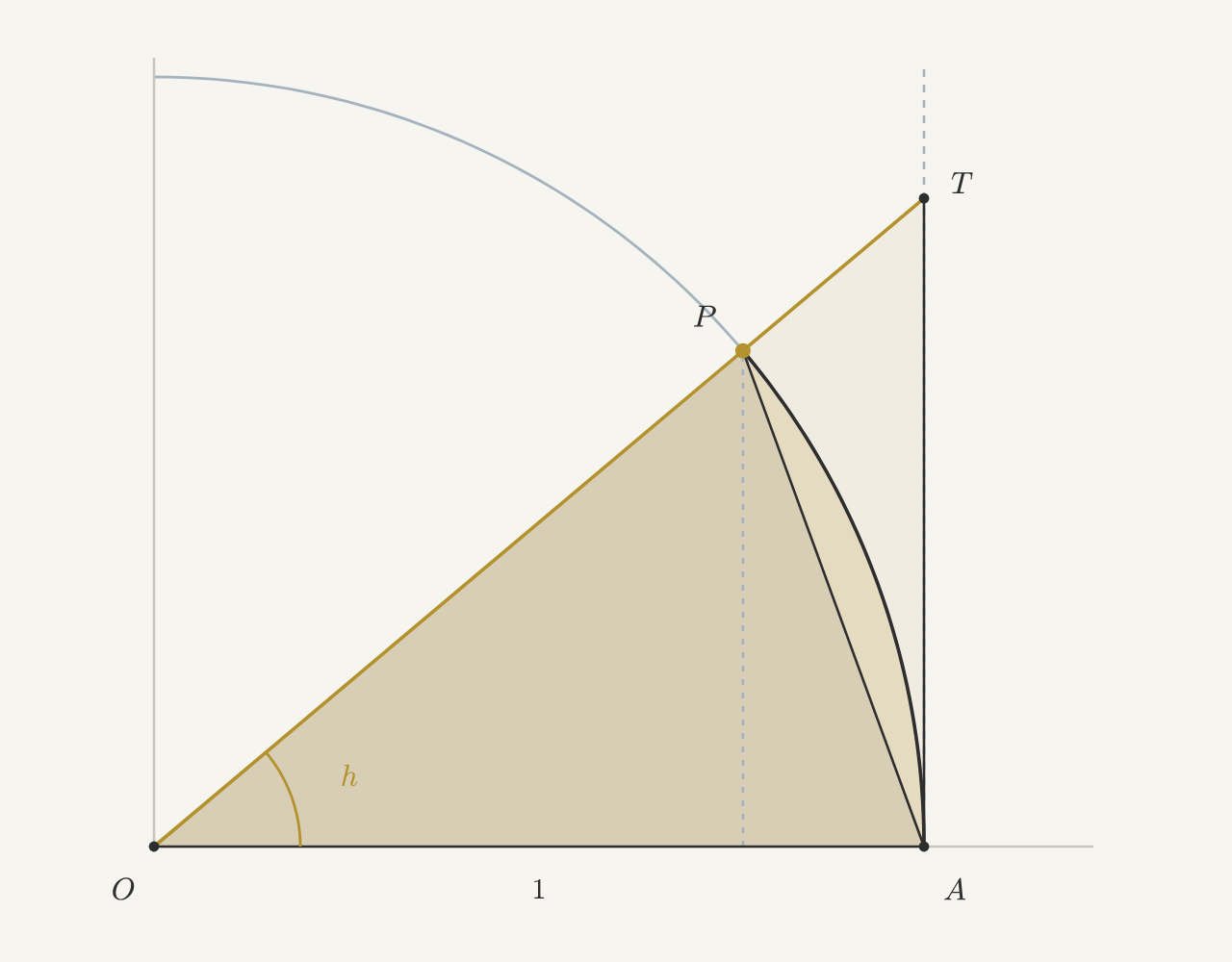
The derivative formulas for sine and cosine come from the geometry of a small angle. Measure angles in radians. For $0 < ℎ < 𝜋 / 2$ , draw the unit circle with center $𝑂$ , the point $𝐴 = (1, 0)$ , and $𝑃 = (c o s ℎ, s i n ℎ)$ . Extend the ray $𝑂 𝑃$ to meet the tangent line $𝑥 = 1$ at $𝑇 = (1, t a n ℎ)$ .

The triangle $𝑂 𝐴 𝑃$ lies inside the circular sector $𝑂 𝐴 𝑃$ , which lies inside the triangle $𝑂 𝐴 𝑇$ . Comparing their areas gives

12 s i n ℎ < 12 ℎ < 12 t a n ℎ .

The sector has area $ℎ / 2$ because its angle is the fraction $ℎ / (2 𝜋)$ of a full circle of area $𝜋$ . This is where radian measure enters.

Figure A.1 The inscribed triangle lies inside the sector, and the sector inside the tangent triangle. Their common base $𝑂 𝐴$ has length one; the triangle heights are $s i n ℎ$ and $t a n ℎ$ . Vary the angle to compare the three areas as $ℎ$ decreases. The area inequalities, rather than the appearance of the picture, establish the limit.

Rearranging the inequalities gives

c o s ℎ < s i n ℎ ℎ < 1 .

As $ℎ \to 0 +$ , the point $𝑃$ approaches $𝐴$ , so $c o s ℎ \to 1$ . The squeeze theorem gives the limit $1$ ; because $s i n ℎ / ℎ$ is even, the same limit holds from the left. Using the circle identity $s i n 2 ℎ + c o s 2 ℎ = 1$ then gives

c o s ℎ - 1 ℎ = - s i n ℎ ℎ s i n ℎ 1 + c o s ℎ ⟶ 0 .

Now the angle-addition identity supplies the derivative:

s i n (𝑥 + ℎ) - s i n 𝑥 ℎ = s i n 𝑥 c o s ℎ - 1 ℎ + c o s 𝑥 s i n ℎ ℎ ⟶ c o s 𝑥 .

The cosine addition identity similarly gives $- s i n 𝑥$ . Thus

(s i n 𝑥)' = c o s 𝑥, (c o s 𝑥)' = - s i n 𝑥 .

The quotient rule gives $(t a n 𝑥)' = 1 / c o s 2 𝑥$ wherever $c o s 𝑥 \neq 0$ . On $(- 𝜋 / 2, 𝜋 / 2)$ , tangent has the inverse $a r c t a n$ , so the inverse derivative rule gives

(a r c t a n 𝑥)' = c o s 2 (a r c t a n 𝑥) = 1 1 + 𝑥 2 .

Here the last equality uses $1 + t a n 2 𝜃 = 1 / c o s 2 𝜃$ .

A.2.3Exponentials and logarithms

Begin with a familiar exponential $𝑎 𝑥$ , where $𝑎 > 0$ . We take the ordinary exponent laws and differentiability of these functions as known from calculus. The addition law separates the difference quotient:

𝑎 𝑥 + ℎ - 𝑎 𝑥 ℎ = 𝑎 𝑥 𝑎 ℎ - 1 ℎ .

Since $𝑎 0 = 1$ , the limit of the last factor is exactly the slope of $𝑎 𝑥$ at zero. So the derivative of an exponential is the exponential itself, multiplied by its slope at zero.

Which base makes that extra factor equal to $1$ ? That base is $𝑒$ : the number $𝑒 \approx 2.71828$ is characterized by

l i m ℎ \to 0 𝑒 ℎ - 1 ℎ = 1 .

We take the existence of this base as known from calculus. The difference-quotient calculation above now gives

𝑑 𝑑 𝑥 𝑒 𝑥 = 𝑒 𝑥 .

The natural exponential $𝑒 𝑥$ has both value $1$ and slope $1$ at zero, and its derivative equals its value everywhere.

The natural logarithm, written $l o g 𝑥$ or $l n 𝑥$ , is the inverse of this exponential. Its domain is $𝑥 > 0$ , and

𝑒 l o g 𝑥 = 𝑥, l o g (𝑒 𝑡) = 𝑡 .

The inverse rule now does the work:

(l o g 𝑥)' = 1 𝑒 l o g 𝑥 = 1 𝑥 .

The exponential addition law also gives $l o g (𝑎 𝑏) = l o g 𝑎 + l o g 𝑏$ for positive $𝑎, 𝑏$ . For another positive base $𝑎$ , write $𝑎 = 𝑒 l o g 𝑎$ and use the chain rule:

𝑎 𝑥 = 𝑒 𝑥 l o g 𝑎, 𝑑 𝑑 𝑥 𝑎 𝑥 = (l o g 𝑎) 𝑎 𝑥 .

Likewise, for a real exponent $𝛼$ and $𝑥 > 0$ ,

𝑥 𝛼 = 𝑒 𝛼 l o g 𝑥, 𝑑 𝑑 𝑥 𝑥 𝛼 = 𝑒 𝛼 l o g 𝑥 𝛼 𝑥 = 𝛼 𝑥 𝛼 - 1 .

This extends the power rule beyond the integer case proved earlier. For integer powers we also have the larger domains already allowed by their algebraic definitions.

One form of the logarithm derivative is particularly useful when integrating. For $𝑥 < 0$ , the chain rule gives $(l o g (- 𝑥))' = (- 1) / (- 𝑥) = 1 / 𝑥$ . Together with the positive case, this says

𝑑 𝑑 𝑥 l o g | 𝑥 | = 1 𝑥 (𝑥 \neq 0), 𝑑 𝑑 𝑡 l o g | 𝑔 (𝑡) | = 𝑔' (𝑡) 𝑔 (𝑡) (𝑔 (𝑡) \neq 0) .

Try this 3. Differentiate $𝑒 - 𝑡 s i n (2 𝑡)$ and $(l o g 𝑡) / 𝑡$ , stating where each formula is valid.

Try this 4. Differentiate $l o g | 1 - 𝑡 2 |$ . On which intervals is this function differentiable? Does a negative value of $1 - 𝑡 2$ prevent us from using the formula?

A.3Integration and the Fundamental Theorem

An integral adds up a rate over an interval. For continuous $𝑓$ , the definite integral $\int 𝑏 𝑎 𝑓 (𝑠) 𝑑 𝑠$ is the limit of sums of values of $𝑓$ times small interval widths. Contributions below zero carry a negative sign. Reversing the bounds reverses the sign, and an interval of zero length gives zero.

Fix $𝑎$ and let the other endpoint vary:

𝐹 𝑎 (𝑡) = \int 𝑡 𝑎 𝑓 (𝑠) 𝑑 𝑠 .

We have defined a function of $𝑡$ . The letter $𝑠$ is a dummy variable which runs through the integral; renaming it does not change the answer. The subscript on $𝐹 𝑎$ records the base point, which stays fixed.

Theorem A.1 (Fundamental Theorem of Calculus). Let $𝑓$ be continuous on an interval $𝐼$ and let $𝑎 \in 𝐼$ . Then $𝐹 𝑎 (𝑡) = \int 𝑡 𝑎 𝑓 (𝑠) 𝑑 𝑠$ satisfies $𝐹' 𝑎 (𝑡) = 𝑓 (𝑡)$ at interior points of $𝐼$ . If $𝐺' = 𝑓$ on $𝐼$ , then for $𝑎, 𝑏 \in 𝐼$ ,

\int 𝑏 𝑎 𝑓 (𝑠) 𝑑 𝑠 = 𝐺 (𝑏) - 𝐺 (𝑎) .

The first statement comes from

𝐹 𝑎 (𝑡 + ℎ) - 𝐹 𝑎 (𝑡) ℎ = 1 ℎ \int 𝑡 + ℎ 𝑡 𝑓 (𝑠) 𝑑 𝑠 .

This is the average value of $𝑓$ over a shrinking interval, so continuity makes its limit $𝑓 (𝑡)$ . For the second statement, $𝐺 - 𝐹 𝑎$ has derivative zero and hence is constant by the mean value theorem. Evaluating that constant at $𝑎$ gives $𝐺 (𝑡) - 𝐹 𝑎 (𝑡) = 𝐺 (𝑎)$ .

A.3.1Which integral are we writing?

An antiderivative of $𝑓$ is a function $𝐺$ with $𝐺' = 𝑓$ . Any two antiderivatives differ by a constant on an interval, since their difference has derivative zero. The indefinite integral notation records the whole family:

\int 𝑓 (𝑡) 𝑑 𝑡 = 𝐺 (𝑡) + 𝐶 .

There are no bounds because no value or base point has yet been selected. By contrast, a definite integral with fixed bounds gives a number, while a variable bound gives a particular function. For the same integrand,

\int 2 𝑡 𝑑 𝑡 = 𝑡 2 + 𝐶, \int 20 2 𝑠 𝑑 𝑠 = 4, \int 𝑡 0 2 𝑠 𝑑 𝑠 = 𝑡 2 .

The last expression selects the antiderivative which is zero at $𝑡 = 0$ . There is no missing $+ 𝐶$ in a definite integral: its bounds have already fixed its value. To describe every antiderivative, we add a constant outside the definite integral:

𝑦 (𝑡) = 𝐶 + \int 𝑡 0 𝑓 (𝑠) 𝑑 𝑠 .

This will be our default form when zero belongs to the interval under consideration. In this form $𝐶 = 𝑦 (0)$ . There is nothing mandatory about zero, however. We can choose any base point $𝑎$ in the interval and write

𝑦 (𝑡) = 𝐶 + \int 𝑡 𝑎 𝑓 (𝑠) 𝑑 𝑠, 𝐶 = 𝑦 (𝑎) .

Changing the base point changes the constant needed to describe the same function. An initial condition $𝑦 (𝑡 0) = 𝑦 0$ suggests an especially convenient choice:

𝑦 (𝑡) = 𝑦 0 + \int 𝑡 𝑡 0 𝑓 (𝑠) 𝑑 𝑠 .

If we keep another base point $𝑎$ , then $𝐶 = 𝑦 0 - \int 𝑡 0 𝑎 𝑓 (𝑠) 𝑑 𝑠$ . If instead we start from an arbitrary antiderivative $𝐺$ , the formula $𝑦 = 𝐺 + 𝐶$ requires $𝐶 = 𝑦 0 - 𝐺 (𝑡 0)$ . The symbol $𝐶$ does not have a fixed numerical meaning independent of how we write the antiderivative.

For example, the problem $𝑦' = 2 𝑡$ , $𝑦 (1) = 3$ from Chapter 2 can be written in all three ways:

𝑦 (𝑡) = 𝑡 2 + 2 = 2 + \int 𝑡 0 2 𝑠 𝑑 𝑠 = 3 + \int 𝑡 1 2 𝑠 𝑑 𝑠 .

The constants $2$ and $3$ differ because the integrals have different base points. Both expressions describe the same function.

An integral also defines an explicit function when no elementary antiderivative is available. For instance,

𝐻 (𝑡) = \int 𝑡 0 𝑒 - 𝑠 2 𝑑 𝑠

is a particular function with $𝐻 (0) = 0$ and $𝐻' (𝑡) = 𝑒 - 𝑡 2$ . The integral specifies its value at every $𝑡$ ; an elementary formula is not required. Numerical integration approximates those values, while the Fundamental Theorem gives its derivative exactly.

A.3.2Logarithms and variable endpoints

We defined the logarithm as an inverse function and proved that its derivative is $1 / 𝑥$ . The Fundamental Theorem now identifies its integral representation:

\int 𝑥 1 𝑑 𝑢 𝑢 = l o g 𝑥 - l o g 1 = l o g 𝑥, 𝑥 > 0 .

Thus the inverse of the exponential also measures accumulated area under $1 / 𝑥$ . Notice the base point $1$ . We could not replace it by zero here: the integrand is undefined there and the integral diverges. Base points must respect the interval on which the calculation makes sense.

Finally, combine the Fundamental Theorem with the chain rule. If $𝑢 (𝑡)$ and $𝑣 (𝑡)$ are differentiable and their values lie in the interval of continuity of $𝑓$ , then

𝑑 𝑑 𝑡 \int 𝑣 (𝑡) 𝑢 (𝑡) 𝑓 (𝑠) 𝑑 𝑠 = 𝑓 (𝑣 (𝑡)) 𝑣' (𝑡) - 𝑓 (𝑢 (𝑡)) 𝑢' (𝑡) .

One way to see both terms is to write the integral as $𝐹 𝑎 (𝑣 (𝑡)) - 𝐹 𝑎 (𝑢 (𝑡))$ . No antiderivative formula for $𝑓$ is needed.

Try this 5. Solve $𝑦' = c o s 𝑡$ , $𝑦 (𝜋 / 2) = 3$ . Write the answer as an elementary antiderivative plus a constant, as a constant plus an integral from $0$ to $𝑡$ , and as an integral based at the initial time.

Try this 6. Differentiate $\int 𝑡 2 𝑡 𝑒 - 𝑠 2 𝑑 𝑠$ without evaluating the integral.

A.4Substitution and Integration by Parts

The chain rule says that if $𝐹' = 𝑓$ , then $(𝐹 (𝑔 (𝑡)))' = 𝑓 (𝑔 (𝑡)) 𝑔' (𝑡)$ . Read backward, it gives

\int 𝑓 (𝑔 (𝑡)) 𝑔' (𝑡) 𝑑 𝑡 = 𝐹 (𝑔 (𝑡)) + 𝐶 .

The substitution notation $𝑢 = 𝑔 (𝑡)$ , $𝑑 𝑢 = 𝑔' (𝑡) 𝑑 𝑡$ records this same calculation. Its purpose is to recognize an outer function together with the derivative of its input. For example,

\int 2 𝑡 1 + 𝑡 2 𝑑 𝑡 = \int 𝑑 𝑢 𝑢 = l o g 𝑢 + 𝐶 = l o g (1 + 𝑡 2) + 𝐶, 𝑢 = 1 + 𝑡 2 .

We do not need an absolute value in the final expression because $1 + 𝑡 2 > 0$ . A substitution in a definite integral also changes its bounds:

\int 𝑏 𝑎 𝑓 (𝑔 (𝑡)) 𝑔' (𝑡) 𝑑 𝑡 = \int 𝑔 (𝑏) 𝑔 (𝑎) 𝑓 (𝑢) 𝑑 𝑢 .

For this form of substitution, $𝑓$ continuous and $𝑔$ continuously differentiable suffice; $𝑔$ need not be one-to-one. The identity follows by evaluating $𝐹 (𝑔 (𝑏)) - 𝐹 (𝑔 (𝑎))$ on both sides. Reversals in direction are already accounted for by the signed derivative and bounds.

For a product, $(𝑢 𝑣)' = 𝑢' 𝑣 + 𝑢 𝑣'$ . Integrating and rearranging gives integration by parts:

\int 𝑢 (𝑡) 𝑣' (𝑡) 𝑑 𝑡 = 𝑢 (𝑡) 𝑣 (𝑡) - \int 𝑢' (𝑡) 𝑣 (𝑡) 𝑑 𝑡 .

Indefinite integrals here represent antiderivative families; one arbitrary constant in the final answer accounts for the freedom on both sides. With fixed bounds the precise evaluation is

\int 𝑏 𝑎 𝑢 𝑣' 𝑑 𝑡 = 𝑢 (𝑏) 𝑣 (𝑏) - 𝑢 (𝑎) 𝑣 (𝑎) - \int 𝑏 𝑎 𝑢' 𝑣 𝑑 𝑡 .

The useful choice is one for which differentiating $𝑢$ simplifies it, while integrating $𝑣'$ is possible. For $\int 𝑡 𝑒 𝑡 𝑑 𝑡$ , choose $𝑢 = 𝑡$ and $𝑣' = 𝑒 𝑡$ . Then

\int 𝑡 𝑒 𝑡 𝑑 𝑡 = 𝑡 𝑒 𝑡 - \int 𝑒 𝑡 𝑑 𝑡 = (𝑡 - 1) 𝑒 𝑡 + 𝐶 .

Sometimes both techniques are needed in one calculation. Assignment 2 led to

\int 2 𝑡 3 𝑒 𝑡 2 𝑑 𝑡 .

The exponential suggests $𝑢 = 𝑡 2$ , but we must transform the entire integrand: $2 𝑡 3 𝑑 𝑡 = 𝑡 2 (2 𝑡 𝑑 𝑡) = 𝑢 𝑑 𝑢$ . Thus

\int 2 𝑡 3 𝑒 𝑡 2 𝑑 𝑡 = \int 𝑢 𝑒 𝑢 𝑑 𝑢 = (𝑢 - 1) 𝑒 𝑢 + 𝐶 = (𝑡 2 - 1) 𝑒 𝑡 2 + 𝐶 .

The substitution exposes the product which integration by parts can simplify. Differentiating the final answer checks both steps at once.

Try this 7. Use integration by parts to find $\int 𝑡 l o g 𝑡 𝑑 𝑡$ on $𝑡 > 0$ .

Try this 8. Evaluate $\int 10 𝑡 / (1 + 𝑡 2) 𝑑 𝑡$ by substitution, changing the bounds when you change variables.

A.5Partial Fractions

Sometimes the calculus becomes easy after an algebraic rearrangement. For the logistic equation in Chapter 4 we needed to integrate

1 𝑥 (1 - 𝑥 / 𝐾), 𝐾 > 0 .

Its denominator has two distinct linear factors. Try expressing it as a sum with one factor in each denominator:

1 𝑥 (1 - 𝑥 / 𝐾) = 𝐴 𝑥 + 𝐵 𝐾 - 𝑥 .

Multiplying by $𝑥 (𝐾 - 𝑥)$ turns the rational identity into a polynomial identity:

𝐾 = 𝐴 (𝐾 - 𝑥) + 𝐵 𝑥 = 𝐴 𝐾 + (𝐵 - 𝐴) 𝑥 .

Matching the constant and linear coefficients gives $𝐴 = 𝐵 = 1$ . We have therefore reduced the integral to

\int 𝑑 𝑥 𝑥 (1 - 𝑥 / 𝐾) = l o g | 𝑥 | - l o g | 𝐾 - 𝑥 | + 𝐶 .

The minus sign in the second logarithm comes from the derivative of $𝐾 - 𝑥$ . Differentiation verifies the decomposition and its integral. The answer applies on each interval avoiding $0$ and $𝐾$ ; constants on different intervals need not agree.

The general method follows the factorization of the denominator. First use polynomial division if the numerator's degree is at least the denominator's. For the remaining proper fraction, each linear factor $𝑥 - 𝑎$ contributes a term $𝐴 / (𝑥 - 𝑎)$ . A repeated factor $(𝑥 - 𝑎) 𝑚$ requires all powers through $𝑚$ :

𝐴 1 𝑥 - 𝑎 + 𝐴 2 (𝑥 - 𝑎) 2 + \dots + 𝐴 𝑚 (𝑥 - 𝑎) 𝑚 .

A quadratic factor $𝑞 (𝑥)$ with no real root requires a linear numerator $(𝐵 𝑥 + 𝐶) / 𝑞 (𝑥)$ ; if it is repeated, include such a numerator over each power of $𝑞$ . Multiply by the common denominator and match coefficients to find the unknown constants.

Linear-factor terms integrate using powers and logarithms. For a single irreducible quadratic, split its numerator into a multiple of $𝑞'$ and a constant. The first part integrates to a logarithm; completing the square in the remaining part leads to arctangent. The basic identity is

\int 𝑑 𝑥 (𝑥 - 𝑏) 2 + 𝑎 2 = 1 𝑎 a r c t a n 𝑥 - 𝑏 𝑎 + 𝐶, 𝑎 > 0,

which follows by substitution and the arctangent derivative. More elaborate repeated-quadratic integrals need further reductions; the linear factors and single quadratics cover the calculations we need here.

Partial fractions does not introduce a new differentiation rule. It rewrites a rational function until the derivatives we already understand become visible.

Try this 9. Decompose and integrate $1 / [𝑥 (𝑥 + 1)]$ . State the intervals on which your antiderivative formulas apply.

Try this 10. Find an antiderivative of $(2 𝑥 + 3) / (𝑥 2 + 2 𝑥 + 5)$ by separating a derivative-of-the-denominator term and then completing the square.

Answers to the Review Questions

1. The derivatives are $2 𝑓 𝑓' 𝑔 + 𝑓 2 𝑔'$ and $𝑓' (𝑔 (𝑥)) 𝑔' (𝑥) 𝑔 (𝑥) + 𝑓 (𝑔 (𝑥)) 𝑔' (𝑥)$ .

2. $(𝑓 - 1)' (2) = 1 / 4$ . The inverse takes input $2$ back to $1$ , so we use the derivative of $𝑓$ at that recovered input.

3. The first derivative is $𝑒 - 𝑡 (2 c o s (2 𝑡) - s i n (2 𝑡))$ , valid for every real $𝑡$ . The second is $(1 - l o g 𝑡) / 𝑡 2$ , valid on $𝑡 > 0$ .

4. The derivative is $- 2 𝑡 / (1 - 𝑡 2)$ on $(- \infty, - 1)$ , $(- 1, 1)$ , and $(1, \infty)$ . The absolute value allows negative values of $1 - 𝑡 2$ ; only its zeros are excluded.

5. All three expressions are

𝑦 (𝑡) = s i n 𝑡 + 2 = 2 + \int 𝑡 0 c o s 𝑠 𝑑 𝑠 = 3 + \int 𝑡 𝜋 / 2 c o s 𝑠 𝑑 𝑠 .

6. The derivative is $2 𝑡 𝑒 - 𝑡 4 - 𝑒 - 𝑡 2$ . Both endpoint derivatives are needed.

7. Choose $𝑢 = l o g 𝑡$ and $𝑣' = 𝑡$ , so $𝑢' = 1 / 𝑡$ and $𝑣 = 𝑡 2 / 2$ . Then

\int 𝑡 l o g 𝑡 𝑑 𝑡 = 𝑡 2 2 l o g 𝑡 - \int 𝑡 2 𝑑 𝑡 = 𝑡 2 2 l o g 𝑡 - 𝑡 2 4 + 𝐶 .

8. Set $𝑢 = 1 + 𝑡 2$ , so $𝑑 𝑢 = 2 𝑡 𝑑 𝑡$ . The new bounds are $1$ and $2$ , giving $12 \int 21 𝑑 𝑢 / 𝑢 = 12 l o g 2$ .

9. $1 / [𝑥 (𝑥 + 1)] = 1 / 𝑥 - 1 / (𝑥 + 1)$ , so an antiderivative is $l o g | 𝑥 | - l o g | 𝑥 + 1 | + 𝐶$ . The intervals are $(- \infty, - 1)$ , $(- 1, 0)$ , and $(0, \infty)$ .

10. The numerator is $(2 𝑥 + 2) + 1$ and the denominator is $(𝑥 + 1) 2 + 4$ . Thus an antiderivative, valid on all of $ℝ$ , is

l o g (𝑥 2 + 2 𝑥 + 5) + 12 a r c t a n 𝑥 + 1 2 + 𝐶 .