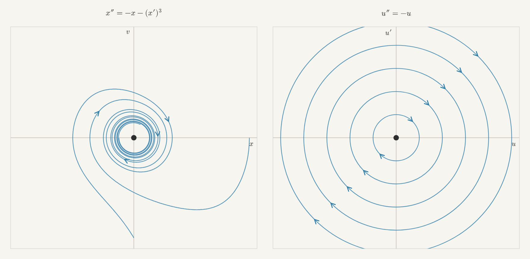
In chapter 11 we met nonlinear systems with several equilibria,
each with its own type. We described those types by looking at pictures.
In this chapter we explain them. Near an equilibrium, a nonlinear system
looks like a linear one, and everything we learned in Part II tells us
what the flow does there.
12.1Slopes and Equilibria
When we can't solve an equation, there is one thing we can always do,
the same thing we did in section 1.2: evaluate the right-hand side.
Let's start with a single equation,
𝑦′=𝑦(1−𝑦).
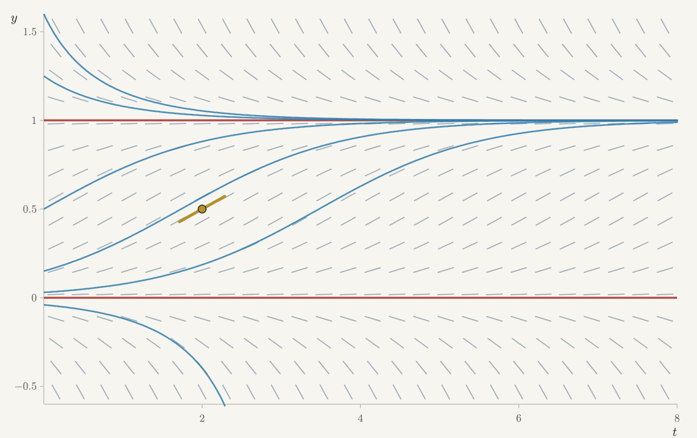
At each height 𝑦, the right-hand side is the slope of every solution
passing through that height. At 𝑦=1/2, for example, the slope is
1/4: a solution passing through 1/2 is rising there at a rate of
1/4.
Figure 12.1 The slope field of 𝑦′=𝑦(1−𝑦). Move the mouse over the picture, or touch
it, to read the slope at that height, and click to release a solution.
Where the slope isn't zero, this one number tells us most of what
happens nearby. Nearby heights have nearly the same slope, so for a short
time, every solution passing nearby rises or falls together at nearly the
same rate. Everything else the equation knows about them is a small
correction. How near is near? Near enough that the slope changes only a
little compared with its value. So the smaller the slope, the closer we
have to stay.
At 𝑦=0 and 𝑦=1 the slope is zero. A solution starting at either
height doesn't move at all: these are the equilibria. Here the slope
tells us nothing about nearby solutions. What they do depends on how the
slopes change as we move away from the equilibrium. Just below 1 the
slopes are small and positive, and just above 1 they are small and
negative, so solutions near 1 move toward it from both sides. How fast
they move depends on how fast the slopes grow as we move away from 1.
For a single equation, the signs of the slopes already tell us whether
nearby solutions approach or leave, as the phase lines of
section 3.5 did. With two equations there is more to
see. Let's look at the system
𝑥′=𝑥(3−𝑥−2𝑦),𝑦′=𝑦(2−𝑥−𝑦).
This is a standard model of two species competing for the same food, with
populations 𝑥 and 𝑦. As populations, only 𝑥≥0 and 𝑦≥0 make
sense, but the equations make sense everywhere, so we will look at the
whole plane.
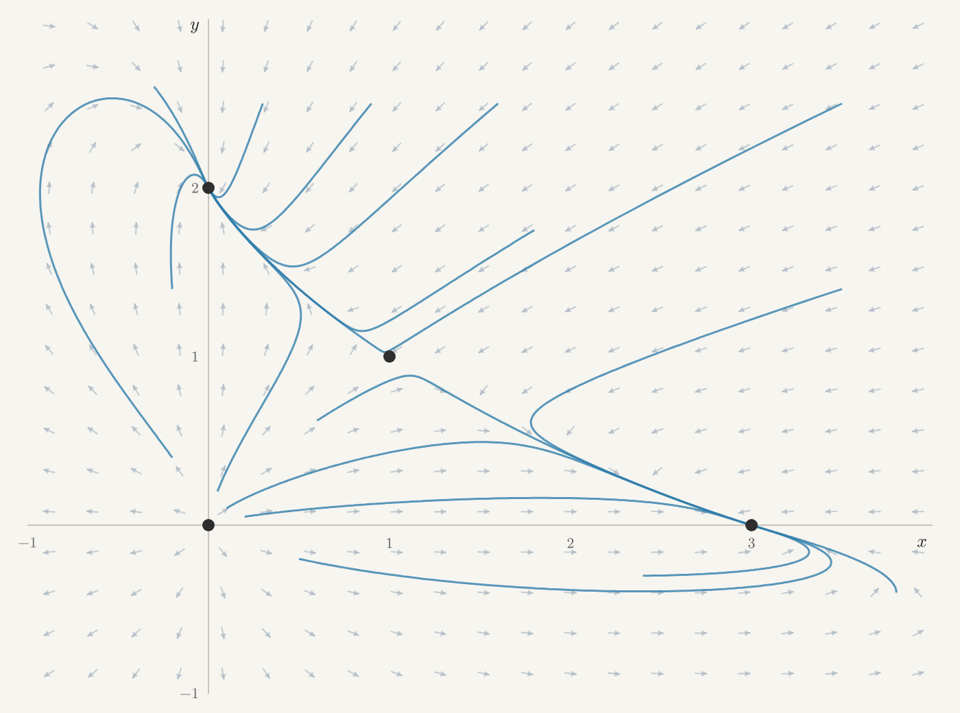
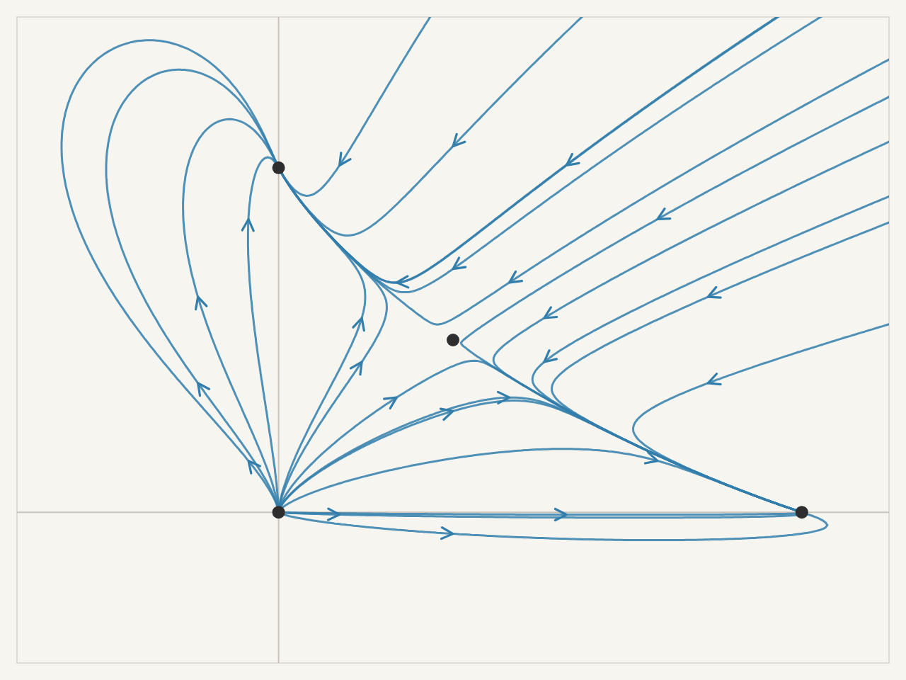
Figure 12.2 Trajectories of 𝑥′=𝑥(3−𝑥−2𝑦), 𝑦′=𝑦(2−𝑥−𝑦). Click to release a state
and follow it.
Release some states and watch where they go. Most come to rest at one of
two points, (3,0) or (0,2), and some leave the picture. Near the
origin, states move away in every direction. Near (1,1), they come in
and then turn away. These special points are the system's equilibria:
states where nothing changes.
At each state (𝑥,𝑦), the two equations give two rates, 𝑥′ and 𝑦′.
Together they form an arrow, which shows the direction and speed of a
state passing through (𝑥,𝑦). This arrow plays the role of the slope.
Where it isn't zero, it tells us most of what happens nearby: for a short
time, nearby states all move in nearly the same direction at nearly the
same speed.
At an equilibrium the arrow is zero, so both rates are zero at once:
𝑥(3−𝑥−2𝑦)=0,𝑦(2−𝑥−𝑦)=0.
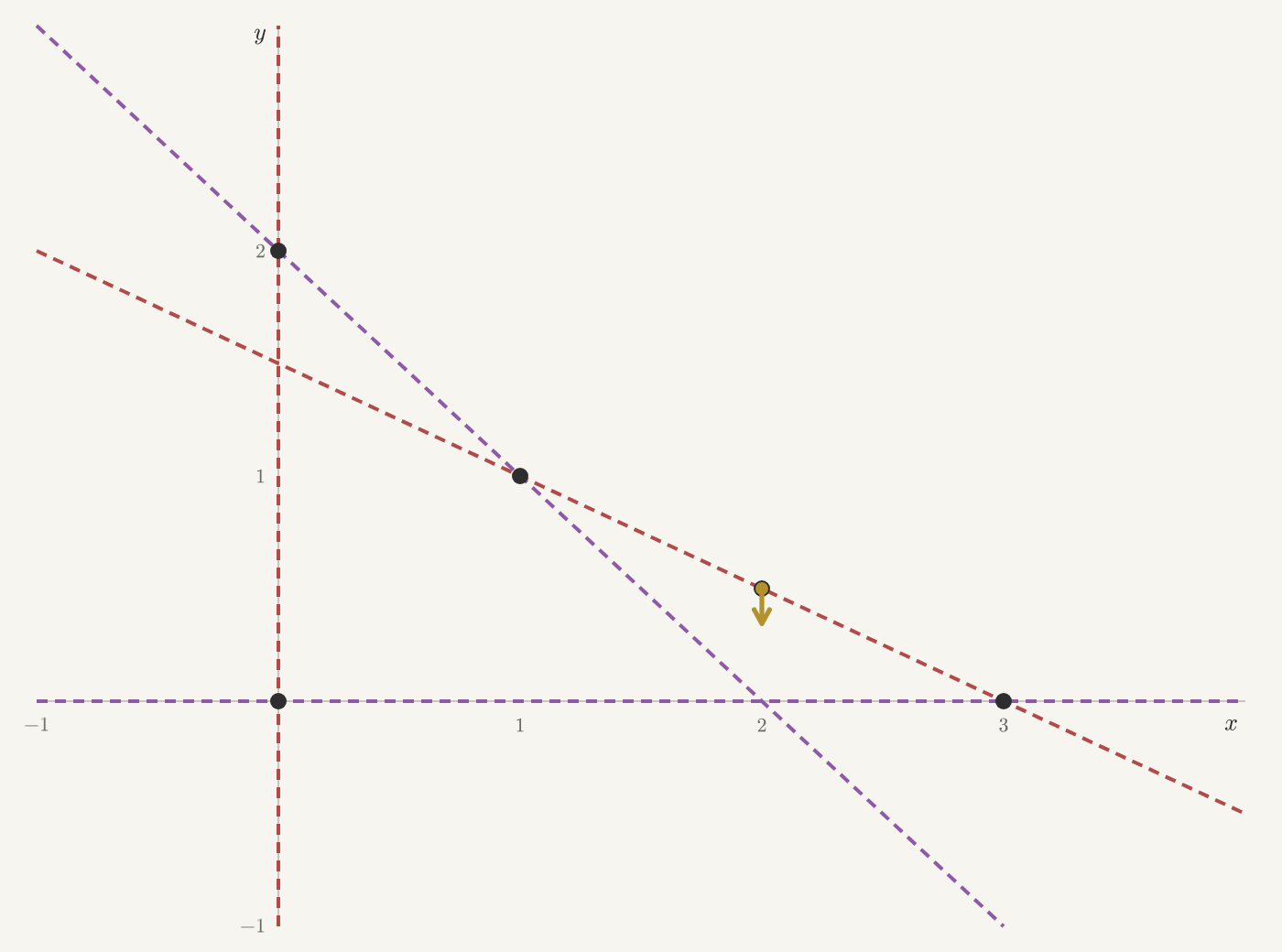
Each rate is a product, so it is zero when either factor is. So 𝑥′=0 on
two lines, 𝑥=0 and 𝑥+2𝑦=3. And 𝑦′=0 on two lines, 𝑦=0 and
𝑥+𝑦=2. Curves like these, where one of the rates is zero, are called
nullclines.
Figure 12.3 The nullclines, red where 𝑥′=0 and violet where 𝑦′=0. Move the mouse
over the picture, or touch it, to see the direction of motion at that
point.
Move the pointer onto a red line. There 𝑥′=0, so the state can't move
left or right, and the arrow points straight up or straight down. On a
violet line, 𝑦′=0, and the arrow points straight left or right. Where a
red line meets a violet one, both rates are zero and the arrow
disappears. These crossings are the equilibria.
So we find the equilibria by pairing each red line with each violet line:
𝑥=0 and 𝑦=0 meet at (0,0).
𝑥=0 and 𝑥+𝑦=2 meet at (0,2).
𝑥+2𝑦=3 and 𝑦=0 meet at (3,0).
𝑥+2𝑦=3 and 𝑥+𝑦=2: subtracting the second from the first gives
𝑦=1, and then 𝑥=1. They meet at (1,1).
As populations, these are no animals, only the second species, only the
first, and both together.
Now look back at the first picture. Near each equilibrium, the flow looks
like one of the linear flows from Part II. The origin looks like a
source, (3,0) and (0,2) look like sinks, and (1,1) looks like a
saddle.
12.2Zooming In on an Equilibrium
Near 𝑦=1, solutions of 𝑦′=𝑦(1−𝑦) approach from both sides, and how
fast they approach depends on how the slopes change near 1. Let's zoom
in on the slope field there. We zoom in only on the heights, and leave
time as it is.
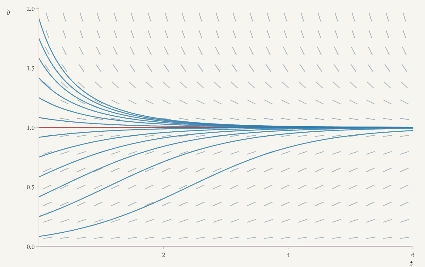
Figure 12.4 The slope field and solutions of 𝑦′=𝑦(1−𝑦) near the equilibrium 𝑦=1.
Move the slider to zoom in on the heights near 1; the time axis stays
the same.
At first the picture is lopsided. Below 1, the slopes level off and
return to zero at the other equilibrium, 𝑦=0. Above 1, they keep
getting steeper. As we zoom in, the lopsidedness disappears, and past a
certain point, zooming in further hardly changes the picture at all.
Let's find the equation of that picture.
First we put the equilibrium at zero by measuring heights from it:
𝑢=𝑦−1.
The equilibrium 𝑦=1 becomes 𝑢=0, and a height close to the
equilibrium has 𝑢 small. Since 𝑢 and 𝑦 differ by a constant, they
change at the same rate: 𝑢′=𝑦′. So substituting 𝑦=1+𝑢,
𝑢′=(1+𝑢)(1−(1+𝑢))=(1+𝑢)(−𝑢)=−𝑢−𝑢2.
There is no constant term, and there couldn't be: at the equilibrium
𝑢=0, nothing changes, so 𝑢′ must be 0 there.
Now compare the two terms that are left. When 𝑢 is about 0.01, the
term −𝑢 is about 0.01, but 𝑢2 is about 0.0001, a hundred times
smaller. The closer we zoom in, the more lopsided this gets. So near the
equilibrium, we drop 𝑢2 and keep
𝑢′≈−𝑢.
This is called the linearization of 𝑦′=𝑦(1−𝑦) at 𝑦=1. It says
that a small distance 𝑢 above or below 1, the slope is about −𝑢.
Its solutions are 𝑢=𝑢0𝑒−𝑡, so near 1, the distance from the
equilibrium shrinks by a factor of 𝑒 every unit of time. And this is
why the zoomed picture stops changing: if 𝑢(𝑡) solves 𝑢′=−𝑢, then so
does 𝑘𝑢(𝑡) for any number 𝑘, so the slope field of 𝑢′=−𝑢 looks the
same at every scale.
Let's put the two side by side.
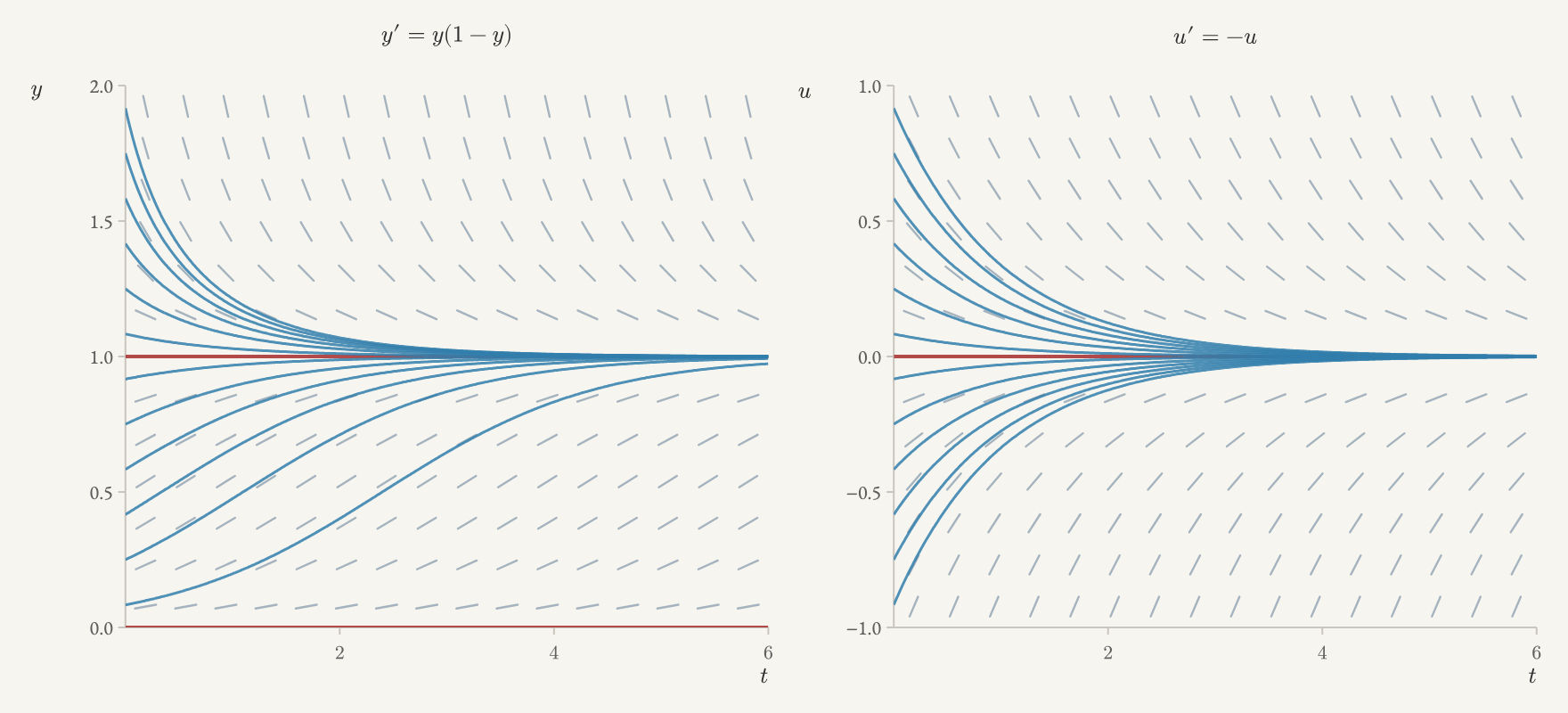
Figure 12.5 Left: the slope field and solutions of 𝑦′=𝑦(1−𝑦) near 𝑦=1. Right:
the slope field and solutions of its linearization 𝑢′=−𝑢 near 𝑢=0,
in a window of the same height. Move the slider to zoom both pictures.
In a large window, the two pictures are different: 𝑦′=𝑦(1−𝑦) has a
second equilibrium at 𝑦=0, and its slopes are lopsided, while the
slopes of 𝑢′=−𝑢 are the same above and below. As we zoom in, they
become the same picture.
Now let's do the same with two equations. In the first picture of our
competition model, the flow near (1,1) looked like a saddle.
Figure 12.6 Trajectories of 𝑥′=𝑥(3−𝑥−2𝑦), 𝑦′=𝑦(2−𝑥−𝑦) near the equilibrium
(1,1). Move the slider to zoom in.
As we zoom in on (1,1), the picture settles down here too, and it
settles into a linear saddle. Let's find that linear system the same
way. We measure each population from its equilibrium value,
𝑢=𝑥−1,𝑣=𝑦−1,
so that 𝑢′=𝑥′ and 𝑣′=𝑦′, and substitute 𝑥=1+𝑢 and 𝑦=1+𝑣 into
the right-hand sides. The first equation becomes
Again the constants cancelled: 3−1−2=0 and 2−1−1=0. And again, each
equation is a linear part, such as −𝑢−2𝑣, plus terms such as 𝑢2 and
𝑢𝑣 that multiply two small numbers together. Near the equilibrium these
products are tiny compared with the linear part, so we drop them:
(𝑢𝑣)′≈(−1−2−1−1)(𝑢𝑣).
This linear system is the linearization of our system at (1,1).
Let's put the two side by side.
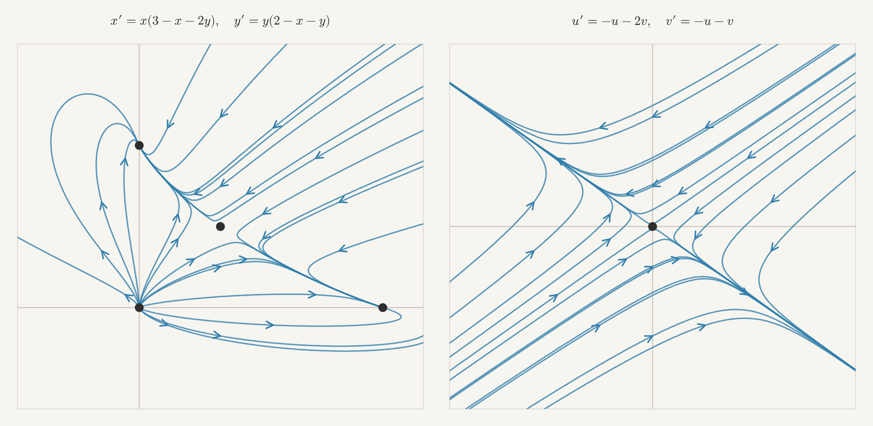
Figure 12.7 Left: trajectories of 𝑥′=𝑥(3−𝑥−2𝑦), 𝑦′=𝑦(2−𝑥−𝑦) near (1,1).
Right: trajectories of its linearization 𝑢′=−𝑢−2𝑣, 𝑣′=−𝑢−𝑣 near
(0,0), in a window of the same size. Move the slider to zoom both
pictures, and click either one to release the same state in both.
In a large window, the two pictures are different: the nonlinear
system has three more equilibria, and the linear one has only the
saddle. As we zoom in, they become the same picture.
Part II tells us exactly what it does. The determinant of its matrix is
(−1)(−1)−(−2)(−1)=−1, which is negative, so it is a saddle. Its
characteristic polynomial is 𝜆2+2𝜆−1, with roots
−1±√2, one negative and one positive. The eigenvector for
−1−√2 is (√2,1), and the eigenvector for −1+√2 is
(√2,−1). So near (1,1), states come in along the direction
(√2,1) and leave along (√2,−1). This is the saddle we saw in
the picture.
12.3The Jacobian Matrix
Multiplying out worked, but it took some algebra, and we would have to
redo it at every equilibrium. Calculus gives a faster way to get the same
linearization. It also explains what we saw in section 12.1:
the slope at a point tells us most of what happens nearby, except at an
equilibrium.
Start with one equation, 𝑦′=𝑓(𝑦). Zooming in on the graph of 𝑓 near
a height 𝑦0 shows its tangent line:
𝑓(𝑦0+𝑢)≈𝑓(𝑦0)+𝑓′(𝑦0)𝑢.
This holds at any height, not just at an equilibrium, and the two terms
do different jobs. The first, 𝑓(𝑦0), is the slope at 𝑦0. The second
says how the slope changes as we move a small distance 𝑢 away. When
𝑓(𝑦0) isn't zero, the first term is the main one, and for small 𝑢
the second is a small correction: nearby heights have nearly the same
slope. But at an equilibrium, 𝑓(𝑦0)=0, and the correction is all
that's left. Measuring heights from the equilibrium, 𝑢′=𝑦′=𝑓(𝑦0+𝑢),
so the linearization at 𝑦0 is
𝑢′=𝑓′(𝑦0)𝑢.
For 𝑦′=𝑦(1−𝑦), we have 𝑓′(𝑦)=1−2𝑦, so 𝑓′(1)=−1. The linearization
at 1 is 𝑢′=−𝑢, just as we found by multiplying out. The −1 that
told us how the slopes change near 1 is the derivative there. At the
other equilibrium, 𝑓′(0)=1, so the linearization is 𝑢′=𝑢, and nearby
solutions move away.
The same works with two equations. Write our system as 𝑥′=𝑓(𝑥,𝑦),
𝑦′=𝑔(𝑥,𝑦). For a function of two variables, zooming in near a point
(𝑎,𝑏) shows its tangent plane. So
The error in each is made of terms like 𝑢2, 𝑢𝑣, and 𝑣2, the same
small products we dropped in section 12.2.
Let's stack these into one statement about the arrow (𝑓,𝑔). Collecting
the terms with 𝑢 and the terms with 𝑣,
(𝑓𝑔)(𝑎+𝑢,𝑏+𝑣)≈(𝑓𝑔)(𝑎,𝑏)+𝑢(𝑓𝑥𝑔𝑥)+𝑣(𝑓𝑦𝑔𝑦),
with all the partial derivatives evaluated at (𝑎,𝑏). The first column
holds the 𝑥-derivatives: how the arrow changes as we move in the 𝑥
direction. The second column holds the 𝑦-derivatives. And 𝑢 times
one column plus 𝑣 times the other is exactly what multiplying a matrix
by (𝑢,𝑣) does:
(𝑓𝑥𝑓𝑦𝑔𝑥𝑔𝑦)(𝑢𝑣)=(𝑓𝑥𝑢+𝑓𝑦𝑣𝑔𝑥𝑢+𝑔𝑦𝑣).
So, writing 𝐹=(𝑓,𝑔), 𝑋0=(𝑎,𝑏), and 𝑈=(𝑢,𝑣),
𝐹(𝑋0+𝑈)≈𝐹(𝑋0)+𝐽𝑈,𝐽=(𝑓𝑥𝑓𝑦𝑔𝑥𝑔𝑦).
This matrix of partial derivatives is called the Jacobian matrix.
Each row comes from one equation, and each column from one variable.
The two terms do the same jobs as before. 𝐹(𝑋0) is the arrow at
𝑋0, and 𝐽𝑈 says how the arrow changes as we move a small
displacement 𝑈 away. Where the arrow isn't zero, it is the main term,
and 𝐽𝑈 is a small correction. At an equilibrium, 𝐹(𝑋0)=0, and 𝐽𝑈
is all that's left. Since 𝑈′=𝑋′, the linearization at an equilibrium
is
𝑈′=𝐽𝑈.
Nothing here depends on having two variables. A system 𝑋′=𝐹(𝑋) in 𝑁
variables 𝑥1,…,𝑥𝑁 has 𝑁 equations 𝑥′𝑖=𝑓𝑖(𝑥1,…,𝑥𝑁).
Its Jacobian is the 𝑁×𝑁 matrix whose entry in row 𝑖 and column
𝑗 is 𝜕𝑓𝑖/𝜕𝑥𝑗: how fast the 𝑖-th rate changes as
we change the 𝑗-th variable. Again 𝐹(𝑋0+𝑈)≈𝐹(𝑋0)+𝐽𝑈, and at
an equilibrium the linearization is 𝑈′=𝐽𝑈.
For our system, 𝑓=3𝑥−𝑥2−2𝑥𝑦 and 𝑔=2𝑦−𝑥𝑦−𝑦2, so
𝐽(𝑥,𝑦)=(3−2𝑥−2𝑦−2𝑥−𝑦2−𝑥−2𝑦).
At (1,1) this is (−1−2−1−1), the same
matrix we found by multiplying out. Evaluating 𝐽 at the other three
equilibria classifies them all. Three of these matrices are triangular,
so their eigenvalues are their diagonal entries.
Equilibrium
Jacobian
Eigenvalues
Type
(0,0)
(3002)
3,2
source
(3,0)
(−3−60−1)
−3,−1
sink
(0,2)
(−10−2−2)
−1,−2
sink
(1,1)
(−1−2−1−1)
−1±√2
saddle
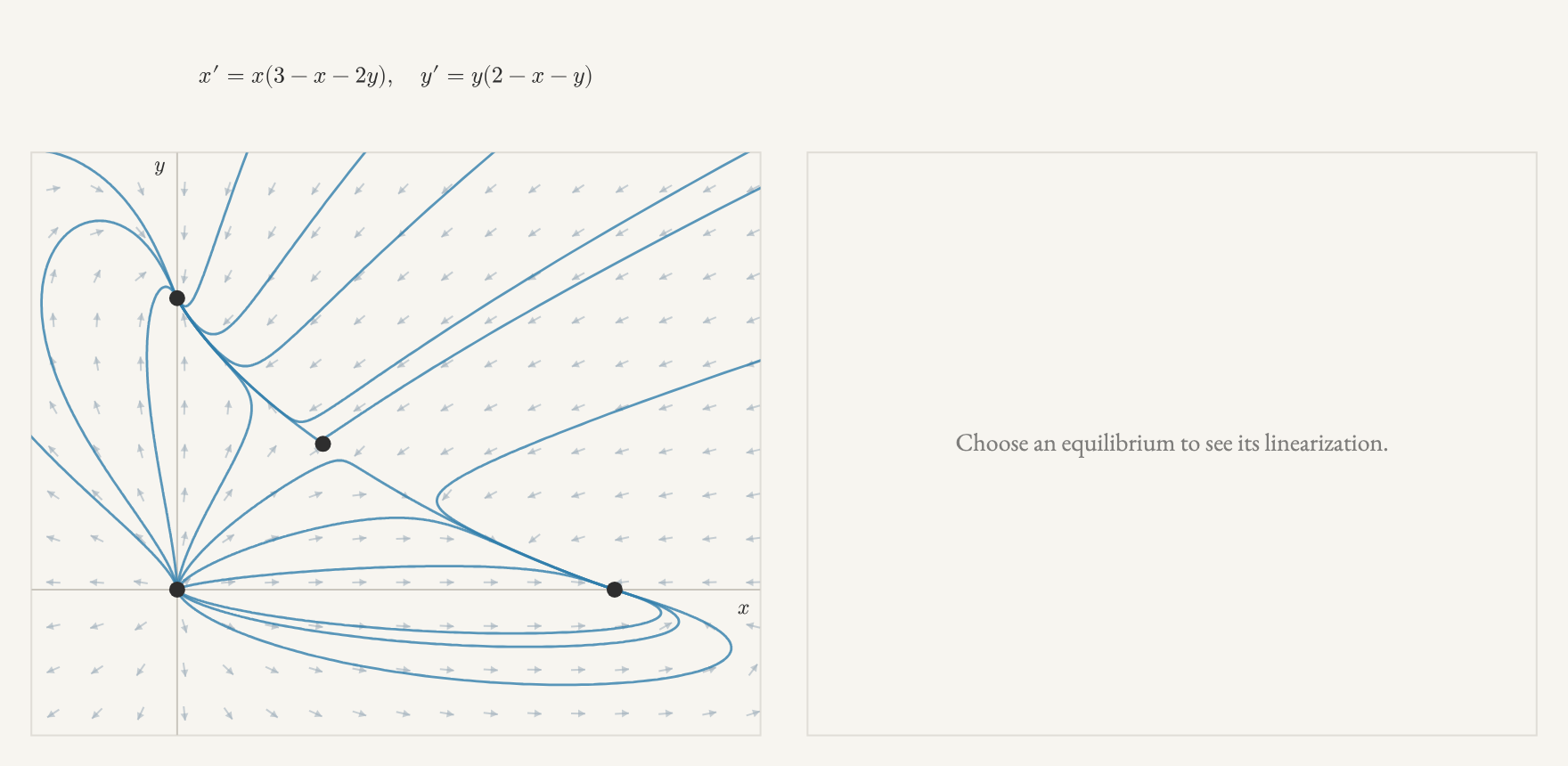
Figure 12.8 Left: trajectories of the competition model. Use the buttons to see the
whole system, or to zoom in on one equilibrium. Right: trajectories of
the linearization 𝑈′=𝐽𝑈 at that equilibrium, in a window of the same
size.
These are the four behaviors we saw in the first picture. The two sinks
are the two ways the competition can end. The saddle is the state where
both species live together, but any small push sends the populations away
from it.
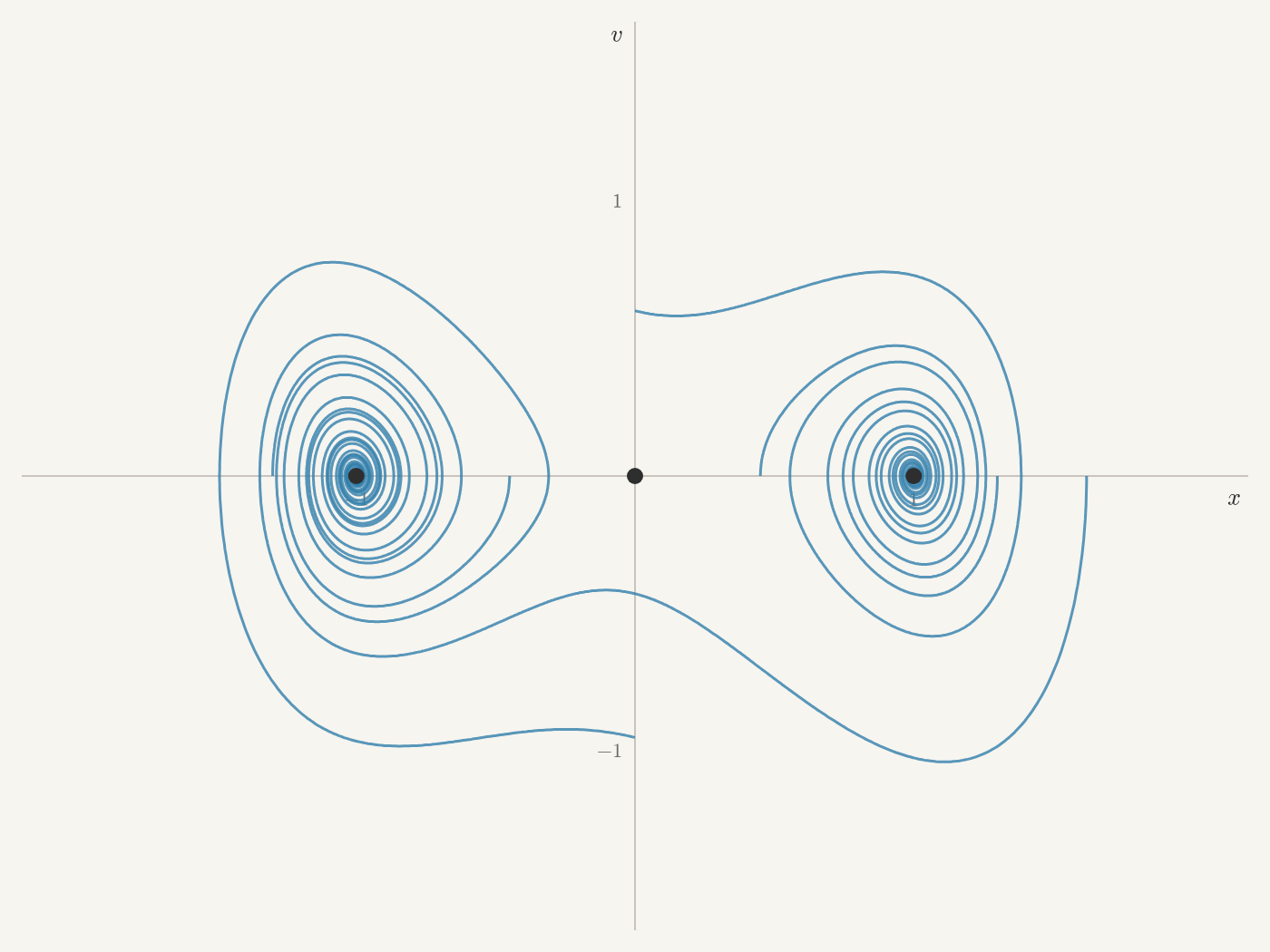
Here is one to try yourself. The double well from chapter 11,
with drag, is 𝑥″=𝑥−𝑥3−𝑐𝑥′, or as a system,
𝑥′=𝑣,𝑣′=𝑥−𝑥3−𝑐𝑣,
with equilibria (−1,0), (0,0), and (1,0).
Figure 12.9 Trajectories of 𝑥′=𝑣, 𝑣′=𝑥−𝑥3−𝑐𝑣. Move the slider to change the drag
𝑐, and click to release a state.
Find the Jacobian, linearize at each of the three equilibria, and check
that the linearizations predict what you see in the picture. Then set the
drag to zero: what does the linearization at (±1,0) predict now?
Now let's try three variables, where the full picture is much more
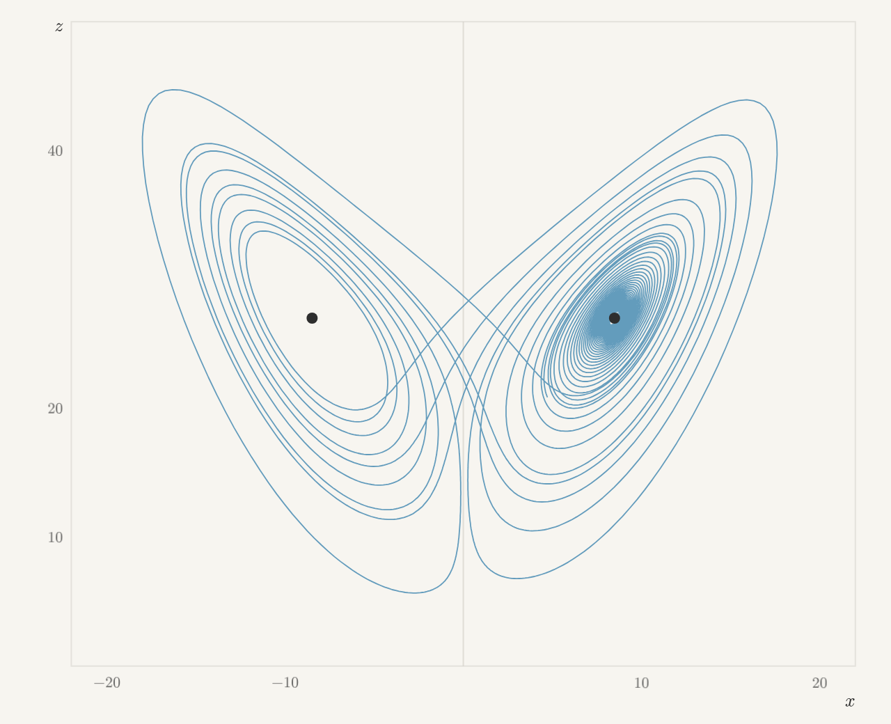
complicated. Recall the Lorenz system from chapter 11:
𝑥′=10(𝑦−𝑥),𝑦′=𝑥(28−𝑧)−𝑦,𝑧′=𝑥𝑦−83𝑧.
Its solutions wind around two lobes. To find the equilibria: 𝑥′=0
gives 𝑦=𝑥. Then 𝑦′=𝑥(28−𝑧)−𝑥=𝑥(27−𝑧), which is zero when 𝑥=0 or
𝑧=27. If 𝑥=0, then 𝑦=0, and 𝑧′=0 gives 𝑧=0. If 𝑧=27, then
𝑧′=𝑥2−72=0 gives 𝑥=±6√2. So there are three equilibria:
(0,0,0) and (±6√2,±6√2,27). The last two sit at the
centers of the two lobes.
The Jacobian is
𝐽(𝑥,𝑦,𝑧)=⎛⎜
⎜
⎜
⎜⎝−1010028−𝑧−1−𝑥𝑦𝑥−83⎞⎟
⎟
⎟
⎟⎠,
and at (6√2,6√2,27) it is
𝐽=⎛⎜
⎜
⎜
⎜
⎜⎝−101001−1−6√26√26√2−83⎞⎟
⎟
⎟
⎟
⎟⎠,
with characteristic polynomial
𝜆3+413𝜆2+3043𝜆+1440.
This cubic has no nice roots, but a computer quickly finds its real
root, 𝜆≈−13.85. Dividing it out leaves a quadratic factor
with no real roots:
𝜆3+413𝜆2+3043𝜆+1440≈(𝜆+13.85)((𝜆−0.094)2+10.192).
So, as in chapter 9, the linearization has an
invariant line, along which states approach quickly at rate −13.85.
It also has an invariant plane, in which states rotate with angular
frequency 10.19 while spiraling slowly outward at rate 0.094. A
state near the equilibrium is pulled onto the plane almost at once, and
then spirals out. Each turn takes about 2𝜋/10.19≈0.62 units
of time, and during one turn its distance from the equilibrium grows by
a factor of only about 𝑒0.094⋅0.62≈1.06. Replacing
(𝑥,𝑦,𝑧) by (−𝑥,−𝑦,𝑧) turns the Lorenz system into itself, so the
same is true at (−6√2,−6√2,27).
Figure 12.10 A solution of the Lorenz system starting close to the equilibrium
(6√2,6√2,27), seen from the side in the (𝑥,𝑧)-plane. Click
to watch again from the start.
This is what we saw in the Lorenz picture: on each lobe, solutions
spiral slowly outward around its center. The linearization explains
that spiral. It says nothing about what happens once a solution has
spiraled far from the center, and that is where it jumps unpredictably
from one lobe to the other.
12.4When Linearization Decides
Linearizing turned each equilibrium of our competition model into a
linear flow we already understood, and the pictures agreed. Does that
always work? Let's start with one equation.
For 𝑦′=𝑓(𝑦), the linearization at an equilibrium 𝑦0 is
𝑢′=𝑓′(𝑦0)𝑢. When 𝑓′(𝑦0) isn't zero, it decides what happens. Near
𝑦0, 𝑓(𝑦0+𝑢)≈𝑓′(𝑦0)𝑢, and for small 𝑢 the error is much
smaller than 𝑓′(𝑦0)𝑢. So 𝑓(𝑦0+𝑢) has the same sign as
𝑓′(𝑦0)𝑢. If 𝑓′(𝑦0)<0, solutions just above 𝑦0 fall and
solutions just below it rise: they approach 𝑦0. If 𝑓′(𝑦0)>0, they
move away.
But when 𝑓′(𝑦0)=0, the linearization is 𝑢′=0, which says that
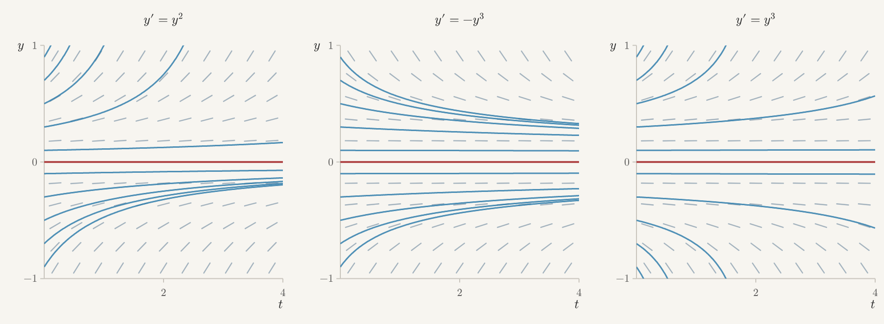
nothing near 𝑦0 moves. Here are three equations, each with an
equilibrium at 0 and linearization 𝑢′=0 there:
𝑦′=𝑦2,𝑦′=−𝑦3,𝑦′=𝑦3.
Figure 12.11 Slope fields and solutions of 𝑦′=𝑦2, 𝑦′=−𝑦3, and 𝑦′=𝑦3. All
three have the same linearization at 0, namely 𝑢′=0.
In none of them does every nearby solution stay put. For 𝑦′=𝑦2, the
slope is positive on both sides of 0: solutions below 0 rise toward
it, and solutions above 0 rise away from it. For 𝑦′=−𝑦3, solutions
approach 0 from both sides. For 𝑦′=𝑦3, they move away on both sides.
The linearization can't tell these apart, because it threw away exactly
the terms that decide. In the Taylor expansion of 𝑓 at 0, 𝑦2 is
the second-derivative term, and ±𝑦3 is the third. When the first
derivative is zero, we have to look at more derivatives.
With two equations, linearization can fail in the same way. When the
Jacobian has determinant zero, the linearization has a whole line of
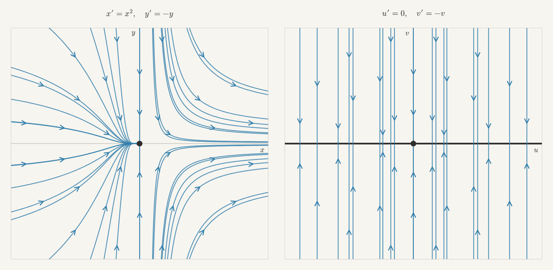
equilibria. Take
𝑥′=𝑥2,𝑦′=−𝑦.
Its only equilibrium is the origin, where the Jacobian is
(000−1), since 2𝑥=0 there. The
linearization 𝑢′=0, 𝑣′=−𝑣 says that every point of the 𝑢-axis is
an equilibrium, and that every state drops straight onto that axis and
stops.
Figure 12.12 Left: trajectories of 𝑥′=𝑥2, 𝑦′=−𝑦. Right: trajectories of its
linearization 𝑢′=0, 𝑣′=−𝑣. Click either picture to release the same
state in both.
The real system has only one equilibrium. What the linearization misses
is the term 𝑥2, a second-derivative term, and on the 𝑥-axis it is
all there is: 𝑥′=𝑥2, which is positive on both sides of 0. So a
state to the left of the 𝑦-axis moves right, toward the origin, while
𝑦=𝑦0𝑒−𝑡 shrinks: it comes into the origin, as at a sink. A state
to the right is pulled toward the 𝑥-axis and then moves away along
it, as on a saddle.
Linearization can also fail at a center. A center is a balancing case.
In the trace–determinant plane, it sits on the half-line between the
spiral sinks and the spiral sources, and any change to the matrix,
however small, can push it to either side. The terms we dropped when we
linearized are small, but they are not zero, and they can do the
pushing.
Here are four springs, each the spring 𝑥″=−𝑥 from Part II with
something extra:
𝑥″=−𝑥−(𝑥′)3,𝑥″=−𝑥+(𝑥′)3,𝑥″=−𝑥−𝑥3,𝑥″=−sin𝑥.
The first has a drag that grows with the cube of the speed, and the
second has the same term pushing instead. The third is a spring that
stiffens as it stretches. The fourth is the pendulum, which fits
because sin𝑥=𝑥−𝑥3/6+⋯ is close to 𝑥 when 𝑥 is small. As
systems, with 𝑣=𝑥′, each has an equilibrium at the origin, and each
extra term has zero derivative there. So all four have the same
Jacobian, (01−10), and the same
linearization: the spring 𝑢″=−𝑢, a center whose trajectories are
circles.
Figure 12.13 Left: trajectories of the chosen spring near the origin, in the
(𝑥,𝑣)-plane. Right: trajectories of their common linearization
𝑢″=−𝑢. Use the buttons to choose the spring, and click to release the
same state in both pictures.
The four springs behave differently. For the first two, follow the
squared distance from the origin, 𝑥2+𝑣2:
(𝑥2+𝑣2)′=2𝑥𝑥′+2𝑣𝑣′=2𝑥𝑣+2𝑣(−𝑥∓𝑣3)=∓2𝑣4.
With the drag, this is never positive: the distance never grows, and it
shrinks except at the moments the state crosses the 𝑥-axis, where
𝑣=0. States spiral slowly inward. With the sign flipped, they spiral
slowly outward. Neither has a single closed loop. The stiffening spring
and the pendulum, on the other hand, go around closed loops near the
origin, as the picture shows. Showing that those loops really close
takes more than linearization.
Again, the dropped terms decide, and here we have to look even further
than for 𝑥2. Each extra term, (𝑥′)3, 𝑥3, or the 𝑥3/6 hidden
in sin𝑥, has zero first and second derivatives at the origin. So the
four springs first differ in their third derivatives.
In both cases, linearization fails because the terms it dropped are the
ones that decide, and we need more derivatives to see them: second
derivatives for 𝑥′=𝑥2, and third derivatives for our springs. In
every other case, linearization gets the picture right. Here is the
general statement, for a system 𝑋′=𝐹(𝑋) with any number of variables.
We'll call it the Linearization Theorem.
Theorem 12.1 (Linearization Theorem). Let 𝑋0 be an equilibrium of 𝑋′=𝐹(𝑋), where 𝐹 has continuous partial
derivatives, and let 𝐽 be the Jacobian matrix of 𝐹 at 𝑋0. Suppose
every real root of the characteristic polynomial of 𝐽 is nonzero, and
every quadratic factor (𝑟−𝑎)2+𝜔2 has 𝑎≠0. Then near 𝑋0,
the flow of 𝑋′=𝐹(𝑋) looks like the flow of its linearization 𝑈′=𝐽𝑈.
More precisely, there is a continuous change of coordinates near 𝑋0
that carries the trajectories of one onto the trajectories of the other,
with time running the same direction.
A continuous change of coordinates can bend the picture, but it can't
tear it. So a saddle stays a saddle, a sink stays a sink, and a source
stays a source. In the plane, the two excluded cases are exactly the ones
we met. A zero root means the determinant is zero. A quadratic factor with
𝑎=0 means the linearization is a center.
The proof of the full theorem is beyond this course. But one part of it
has a short proof, and the proof shows why linearization works. We prove
that part, for sinks in the plane, in section 12.5.
12.5Proving the Linearization Theorem for Sinks
Here is why a sink attracts. We'll take a sink in the plane whose
linearization has two different negative roots, or a rotation with
negative rate.
Write the system as 𝑋′=𝐹(𝑋), where 𝑋=(𝑥,𝑦) is the state and 𝐹(𝑋)
gives the two rates. Let 𝑋0 be the equilibrium, and 𝐽 the Jacobian
matrix there. We measure states from the equilibrium by writing
𝑋=𝑋0+𝑈, so 𝑈 is the displacement from 𝑋0. The tangent-plane
approximation says
𝐹(𝑋0+𝑈)=𝐹(𝑋0)+𝐽𝑈+𝑅(𝑈),
where 𝑅(𝑈) is the error in the approximation: everything that
linearization drops. As we saw in the competition model, it is made of
products of small numbers, like 𝑢2 and 𝑢𝑣. Precisely, there is a
number 𝐶 with |𝑅(𝑈)|≤𝐶|𝑈|2 for all 𝑈 close enough to 0. Since
𝑋0 is an equilibrium, 𝐹(𝑋0)=0, and since 𝑋0 is constant,
𝑈′=𝑋′. So
𝑈′=𝐽𝑈+𝑅(𝑈).
Now we change to good coordinates. Chapter 8 gives an invertible matrix
𝑃 for which 𝐵=𝑃−1𝐽𝑃 is either diagonal or a rotation block. Write
𝑈=𝑃𝑊, so that 𝑊 is the displacement measured in the new coordinates.
Since 𝑃 is constant, 𝑈′=𝑃𝑊′. Substituting into 𝑈′=𝐽𝑈+𝑅(𝑈) and
multiplying by 𝑃−1,
𝑊′=𝑃−1𝐽𝑃𝑊+𝑃−1𝑅(𝑃𝑊)=𝐵𝑊+𝑆(𝑊).
Both pieces change in the same way: put in 𝑃𝑊, apply the piece, then
apply 𝑃−1. The linear part 𝐽 becomes the matrix 𝐵. The leftover
𝑅 becomes a new function, 𝑆(𝑊)=𝑃−1𝑅(𝑃𝑊), of the same kind. Since
𝑃𝑊 is linear in 𝑊, each entry of 𝑆(𝑊) is again built from products
of two small numbers, now 𝑤1 and 𝑤2. So 𝑆 is still small: there is
a number 𝐾 with |𝑆(𝑊)|≤𝐾|𝑊|2 for all 𝑊 close enough to 0.
Now we watch the distance |𝑊| from the equilibrium. It is easier to
work with its square, |𝑊|2=𝑊⋅𝑊, which by the product rule changes
at the rate
(|𝑊|2)′=2𝑊⋅𝑊′=2𝑊⋅𝐵𝑊+2𝑊⋅𝑆(𝑊).
The first term comes from the linearization. Write 𝑊=(𝑤1,𝑤2).
If 𝐵 is diagonal, with negative entries 𝜆1 and 𝜆2, the
first term is 2(𝜆1𝑤21+𝜆2𝑤22). Let 𝜇 be the larger
of 𝜆1 and 𝜆2. Each of 𝜆1,𝜆2 is at most
𝜇, so the first term is at most 2𝜇(𝑤21+𝑤22)=2𝜇|𝑊|2.
If 𝐵 is a rotation block
(𝛼−𝜔𝜔𝛼) with
𝛼<0, the first term is
2(𝑤1(𝛼𝑤1−𝜔𝑤2)+𝑤2(𝜔𝑤1+𝛼𝑤2))=2𝛼|𝑊|2.
The rotation terms cancel, because rotating moves a state around the
equilibrium, not toward or away from it. Let 𝜇=𝛼.
Either way, 𝜇 is a negative number, and the first term is at most
2𝜇|𝑊|2.
The second term comes from the leftover. A dot product is at most the
product of the lengths of its two vectors, so this term is at most
2|𝑊|⋅𝐾|𝑊|2=2𝐾|𝑊|3. Adding the two,
(|𝑊|2)′≤2𝜇|𝑊|2+2𝐾|𝑊|3=2|𝑊|2(𝜇+𝐾|𝑊|).
Now we can see why the equilibrium attracts. The linear part pulls inward
in proportion to |𝑊|2, while the leftover can push outward only in
proportion to |𝑊|3, which is much smaller near the equilibrium.
Precisely, suppose |𝑊|≤−𝜇/(2𝐾), and 𝑊 is close enough to 0 for
our bounds to hold. Then 𝐾|𝑊|≤−𝜇/2, so 𝜇+𝐾|𝑊|≤𝜇/2, and
(|𝑊|2)′≤𝜇|𝑊|2<0.
So a state that starts this close moves closer. It therefore stays this
close, and the inequality keeps holding.
To see that it goes all the way in, multiply by 𝑒−𝜇𝑡. By the
product rule,
(𝑒−𝜇𝑡|𝑊|2)′=𝑒−𝜇𝑡((|𝑊|2)′−𝜇|𝑊|2)≤0,
so 𝑒−𝜇𝑡|𝑊|2 never increases, and
|𝑊(𝑡)|2≤|𝑊(0)|2𝑒𝜇𝑡. Since 𝜇<0, this goes to 0. Because
𝑈=𝑃𝑊, the displacement 𝑈 goes to 0 too: the state approaches the
equilibrium.
For the sink (3,0) of our competition model,
𝐵=(−300−1) and 𝜇=−1. So nearby states
approach (3,0), with |𝑊(𝑡)|≤|𝑊(0)|𝑒−𝑡/2.