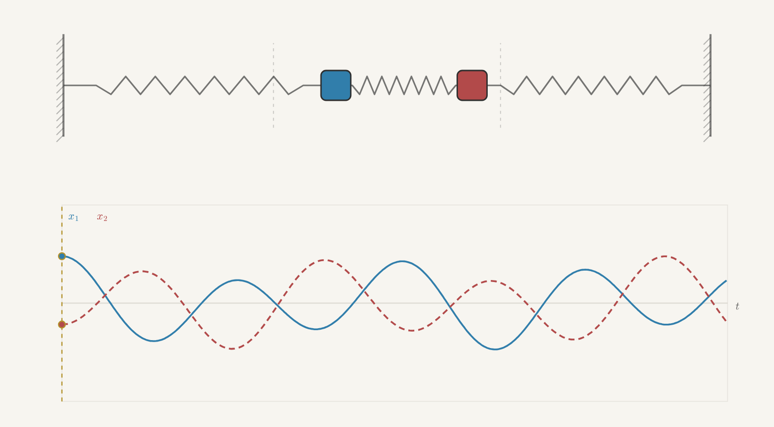
Figure 9.1 In the live figure, drag the two carts to choose a starting displacement,
then let go. Most choices mix two frequencies and change shape as they move.
If the carts begin with equal displacements, however, they retain that shape
and oscillate with 𝜔=1. If they begin with equal and opposite
displacements, they retain the second shape and oscillate with
𝜔=√3.
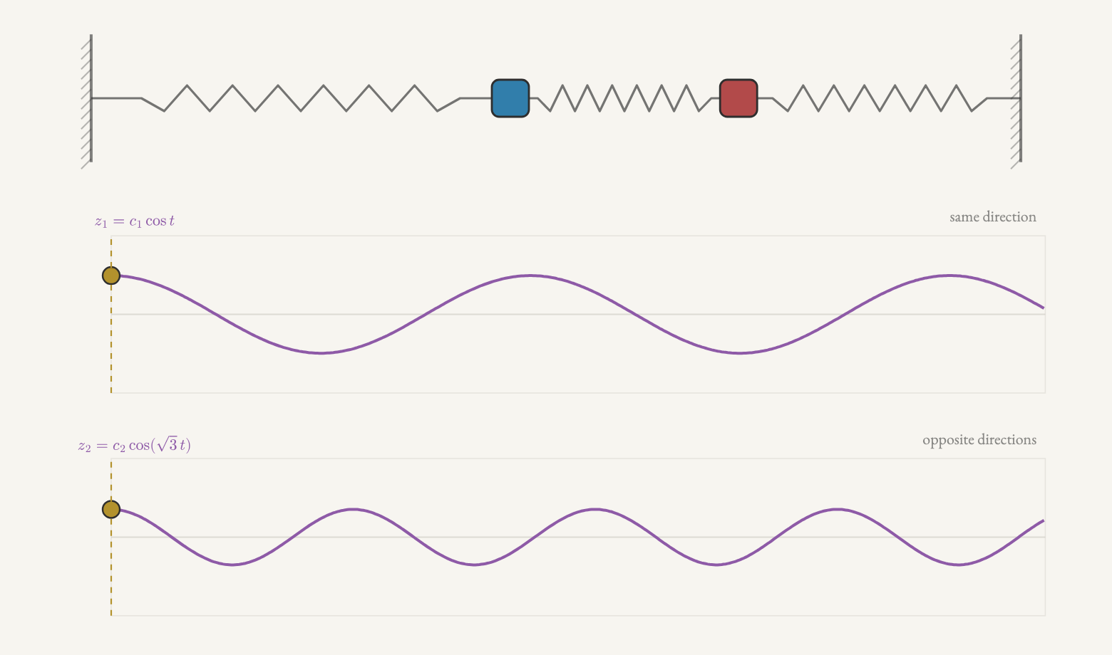
Figure 9.2 The motion shown above is assembled from
𝑐1cos(𝑡) times the in-phase shape and
𝑐2cos(√3𝑡) times the opposite shape. In the live figure, drag the
two amplitude controls. Setting either coefficient to zero isolates one mode; combining
them reconstructs the coupled motion of the carts.
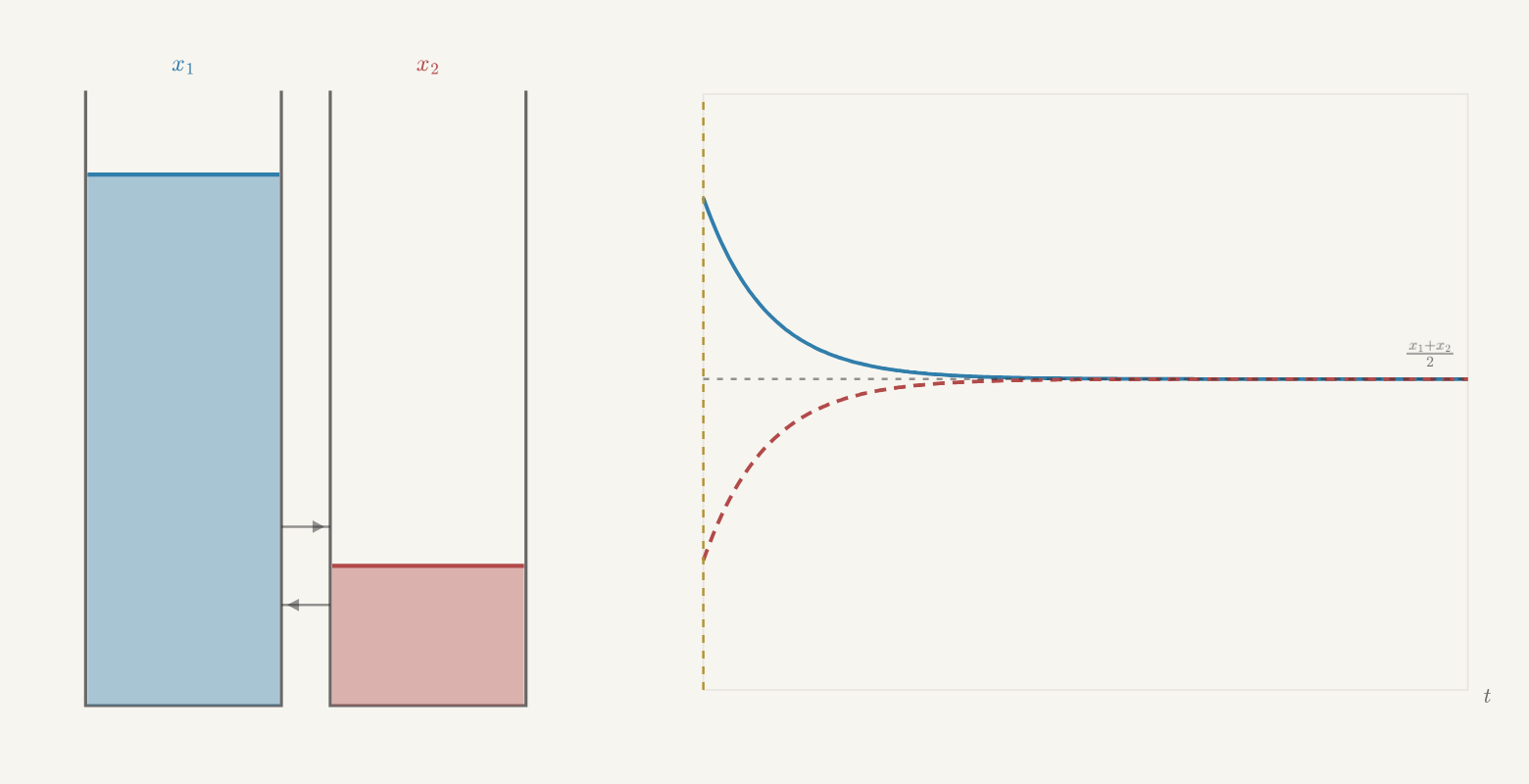
Figure 9.3 In the live figure, drag either brine level. The mean level remains fixed
while the difference between the tanks decays exponentially. These two
patterns---a constant sum and a decaying difference---reconstruct every
approach to equal levels, even though nothing oscillates.
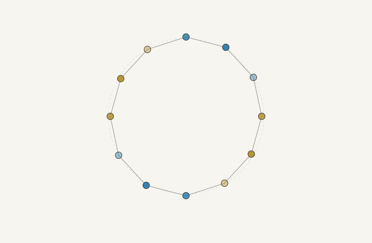
Figure 9.4 In the live figure, move through the modes of twelve coupled masses on a
ring. Higher modes vary more rapidly around the ring and have higher
frequencies; paired modes share a frequency, while the uniform mode has no
restoring force. Switch from 𝑞″=−𝐿𝑞 to 𝑢′=−𝐿𝑢 to make the same spatial
pattern decay instead of oscillate.
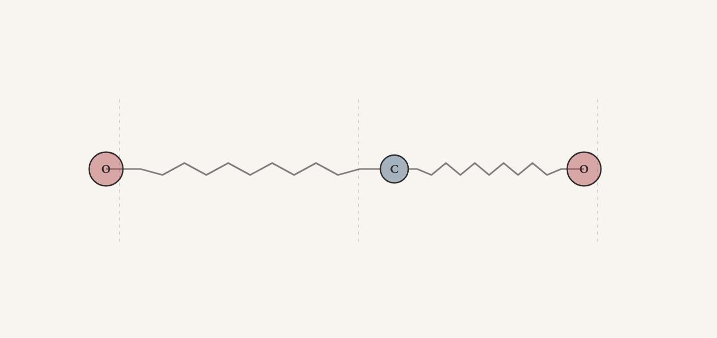
Figure 9.5 The three-mass model is calibrated to the two stretching frequencies of
carbon dioxide. In the live figure, replace 12C with 13C without
changing the fitted bond constants. The predicted antisymmetric frequency shifts to
2282cm−1, compared with the observed
2283.5cm−1. The symmetric frequency does not shift because
the carbon atom remains still in that mode.
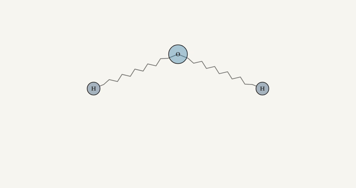
Figure 9.6 The six-coordinate calculation uses water's bent geometry and published
force constants in 𝐾𝑣=𝜔2𝑀𝑣. Three zero eigenvalues correspond to
rigid motions of the molecule, leaving the three vibrational modes shown.
After fitting H2O, keep the same force constants and change only the
isotope masses: the resulting D2O and HDO frequencies agree with the
observed values to about one percent.
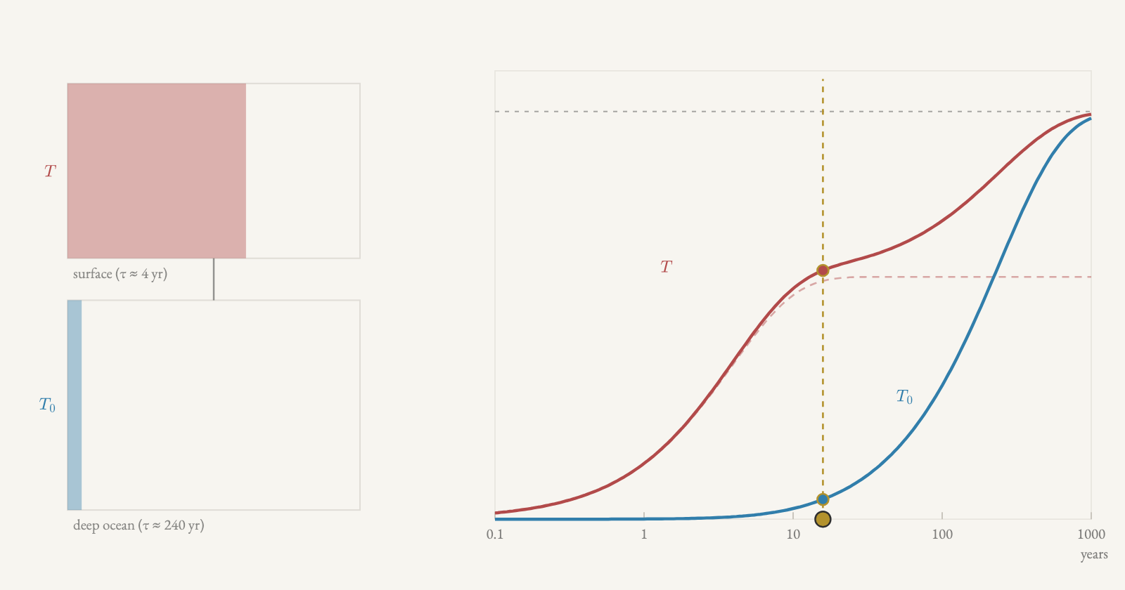
Figure 9.7 In the live figure, drag the marker along the logarithmic time axis after a
step of forcing. The two-box ocean--atmosphere model responds on two time
scales: the surface adjusts over about four years while the deep ocean changes
little, then both boxes continue warming together over roughly two and a half
centuries. The surface completes about 60% of its eventual warming during
the fast part.
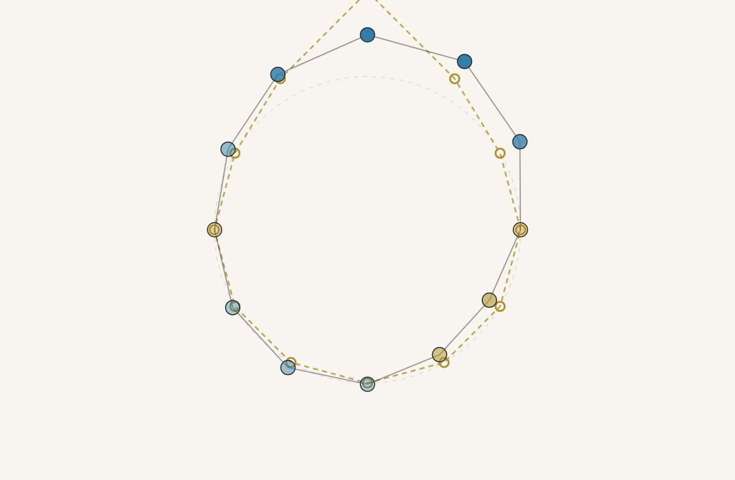
Figure 9.8 In the live figure, drag a mass to create the gold target shape, then choose
how many of the lowest-frequency modes to retain. A few modes recover the broad, smooth
part of the shape. Reproducing the sharp corner requires the higher-frequency
modes as well.
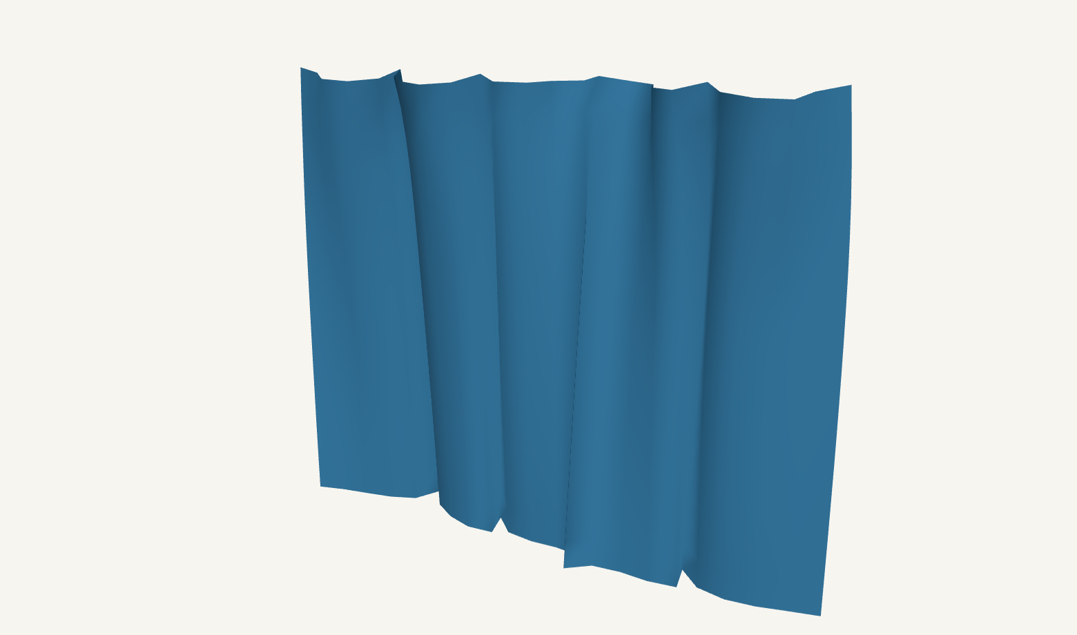
Figure 9.9 This curtain contains a few hundred point masses joined by structural and
shear constraints. Gravity and a light breeze move those masses in real
time; switch views to see the network beneath the rendered surface. Models
of this kind are fast enough for interactive animation, but this example is
not fitted to the behavior of a particular fabric. Drag the figure to orbit
around it.
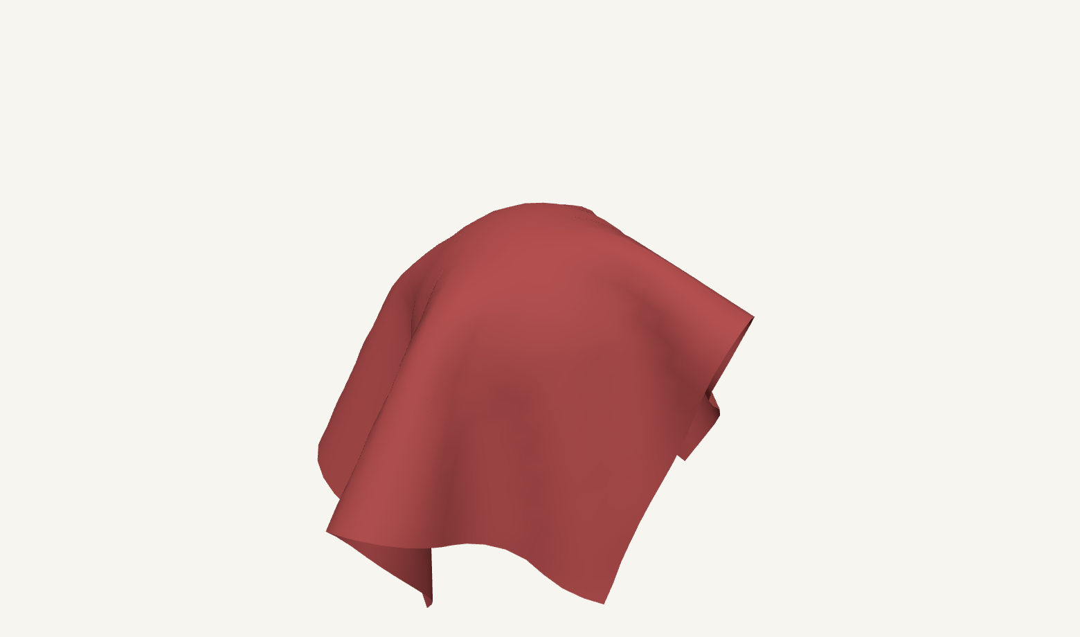
Figure 9.10 Drop the square sheet onto the sphere. Any mass which enters the sphere is
pushed back to its surface and loses most of its speed on contact. Masses
which are far apart on the sheet are also kept from passing through one
another, allowing the folds to stack as the cloth settles. Replay the drop,
switch to the mass-and-spring view, or drag to orbit around the final drape.