Building and Exploring Models
In the last two chapters, we learned how to find solutions to differential equations and how to understand their behavior without finding a formula. But where do the equations come from? If we begin with a question about the world, how do we decide which equation to write?
This is the task of mathematical modeling. We begin by identifying the quantities that seem relevant to our question. Then we decide which changes we need to follow and which quantities we can reasonably treat as constant. Using these ingredients and their derivatives, we try to turn an ordinary description of what is happening into a precise mathematical relationship.
There is an art to these choices. The same description may suggest several equations, and a quantity we treat as constant for one question may need to vary for another. Our aim is to build a model simple enough that we can understand it and make predictions with it, but detailed enough to capture the behavior that matters. Once we have an equation, mathematics tells us what it implies. We can then compare those consequences with observations and use what we learn to revise our choices.
We will begin by returning to Newton's law of cooling, this time slowing down to examine how we build the model. Then we will investigate population growth, letting measurements guide us from a simple model to a more complicated one, before adding harvesting. Elsewhere in the chapter, models of interacting populations, epidemics, and moving springs will ask us to follow more quantities and relate them in new ways. The chapter closes with a climate appendix, where we apply the same modeling approach to Earth's temperature. Ecology, climate, and mechanics will keep returning throughout the book as we develop the mathematics their models lead us to.
4.1Newton's Law of Cooling
Suppose we leave a hot cup of coffee on the table and want to know how warm it will be twenty minutes from now. What quantities might matter? The coffee's current temperature matters, of course. But so does the temperature of its surroundings: the same coffee would cool differently in a warm kitchen and a cold garage.
Let us begin with those two quantities: the temperature of the coffee and the temperature of the room. Which should we treat as variables, and which as constants?
Over twenty minutes, the coffee's temperature may change substantially,
while the room's temperature changes very little. So a reasonable first
choice is to let the coffee's temperature be a function
These are choices about our model. Over a single second, we might reasonably treat both temperatures as nearly constant. Over a whole day, the room may warm and cool enough that we need to follow its temperature too. We choose what to hold fixed by considering the time scale and the question we want to answer.
Now we have our ingredients. What can we say about how they are related? A cup hotter than the room cools down, a cup colder than the room warms up, and a larger temperature difference produces a faster change. The quantity
therefore seems useful: its sign tells us which way the temperature should change, and its magnitude tells us how far the coffee is from matching its surroundings.
But “a larger difference produces a faster change” does not tell us exactly how much faster. We have to make a choice. One simple possibility is proportionality: doubling the temperature difference doubles the rate of change. With the sign chosen so that hot coffee cools, this gives
Why do we need the proportionality constant
Thus
Let us check the equation against the observations that motivated it.
When
We have recovered Newton's law of cooling, which we already solved in chapter 2:
Once we have reason to trust this model---for example, because we have seen
it agree with measurements in many situations---we can put it to work. But
our formula still contains
Fortunately, we do not need to derive
This is a very useful feature of modeling. We began by wanting an entire function---the coffee's future temperature---but the model reduced what we needed to learn to finitely many numbers. A few measurements determine those numbers, and the equation supplies the rest of the history. In the problems, you will use two measurements of a cooling cup of coffee to predict a third.
Try this with the measurements in Figure figure 4.1. Here we have more
than two observations, so we can also see how well one choice of
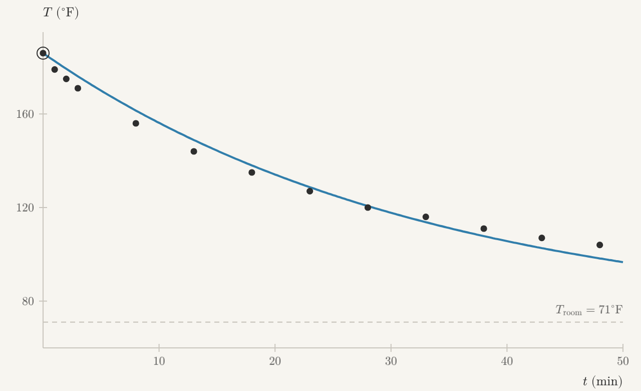
Of course, determining the constant assumes that we have chosen a suitable model. Let us now turn to population growth, where measurements will help us both choose the constants and investigate whether the equation itself needs to change.
4.2Population Growth
How can we predict the size of a growing population? Let us begin with a
population living where food and space are plentiful, and try to describe
its growth with a single quantity: the amount of population present,
4.2.1From Exponential to Logistic Growth
What determines how quickly this quantity changes? New individuals are born, while others die. For a first model, suppose each individual makes approximately the same average contribution to the population's net growth. Then twice as many individuals should produce twice as much net growth over the same short interval. As with cooling, a simple way to express this assumption is proportionality:
The coefficient
Over time, the conditions in which a population lives can change, and its growth rate can change with them. In the United States, the annual birth rate is estimated to have been about 50 births per 1,000 people around 1800; in 2024 it was 10.7. Over those centuries, family life, economic conditions, and expectations about having children changed enormously as the country shifted from a predominantly rural society toward an urban one. Births are only one contribution to population growth---deaths and migration matter too---but even this one contribution is clearly something we cannot treat as constant forever. (Historical estimates; 2024 measurements.)
But we may not need to describe centuries of change. Over a shorter
window---perhaps a few hours for a yeast culture, or a decade for a human
population---the conditions controlling growth may change relatively little
while the population itself changes appreciably. This gives us a reason to
try treating
The units work just as they did for cooling. Since
We already know the solution. If
For
In 1913, Tor Carlson measured the amount of yeast growing in brewer's wort at hourly intervals. Let us imagine watching his experiment as it happens. We have seen the first six measurements, taken an hour apart, and want to use them to build a prediction.
The first measurement gives
Just as with the coffee, the initial measurement fixes one constant, leaving
a single parameter for us to determine. Here it is
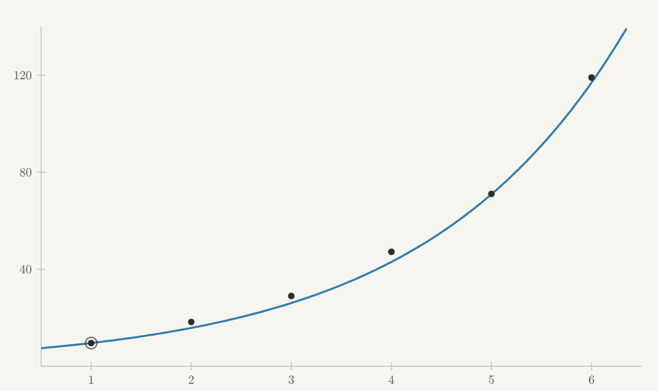
This looks promising! One constant describes the rapid growth quite well. We have done more than draw a curve through measurements: we have chosen a differential equation, used the measurements to determine its remaining parameter, and obtained a function we can evaluate at future times.
But those future values are predictions. To find out whether they are useful, we have to let the experiment continue.
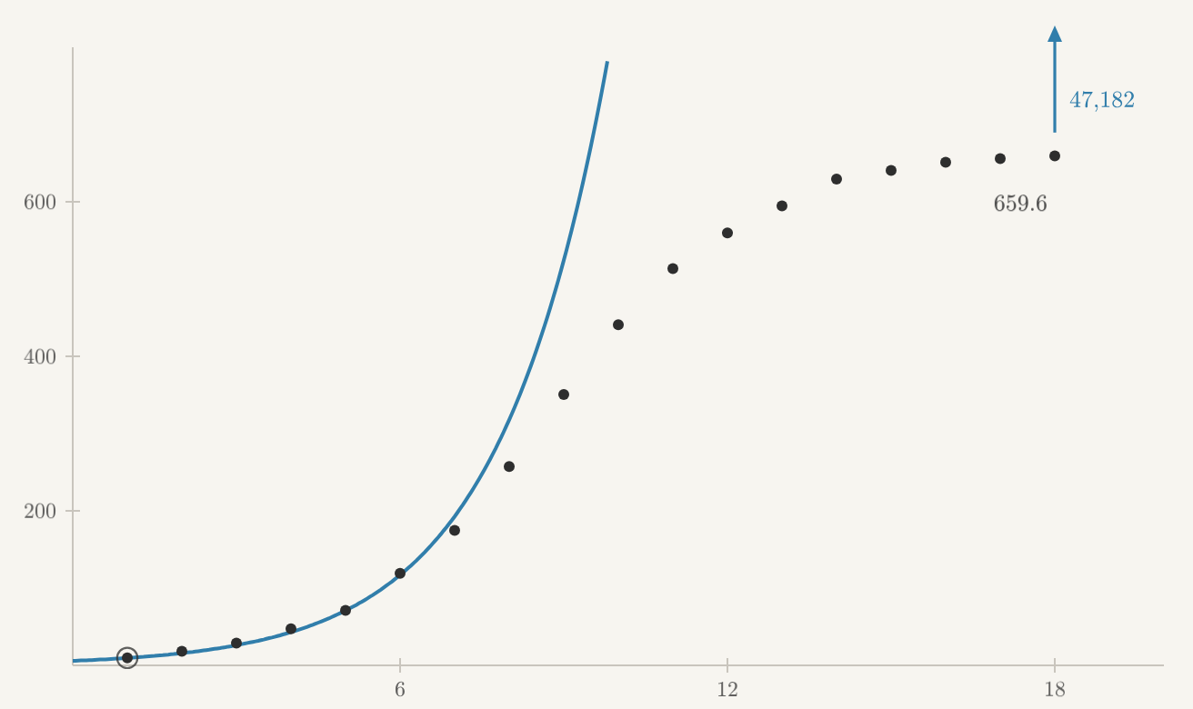
At hour
while Carlson measured
The same model that worked well over a few hours has failed over a longer interval. And adjusting its one constant cannot fix the problem. We need to reconsider the assumption that each unit of population keeps contributing the same net growth per unit time.
Can we use the measurements to check our assumption? We said that each unit of population contributes the same net growth per unit time. To investigate that contribution, divide the total growth rate by the amount of population present:
This is called the per-capita growth rate. Our exponential model says
that it equals the constant
We do not have measurements of
To estimate the growth per unit of population, we also need the amount of
yeast present during that interval. It changes from
We can compute this number for each pair of consecutive measurements, then plot it against the average amount of yeast present.
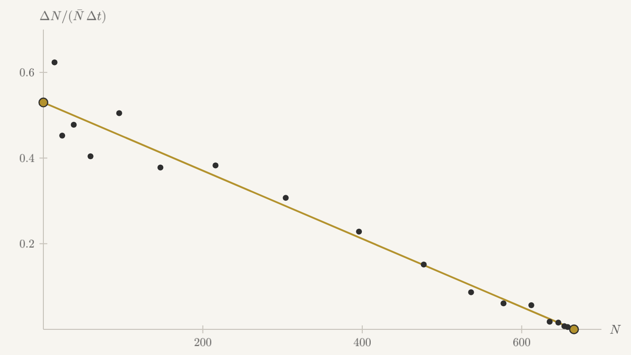
The data suggest a way forward! The per-capita rate is not constant, but its decrease looks approximately linear. We could try many curves through these points; a line is a simple next choice.
Let
Multiplying by
Notice what we have changed. The growth per unit of population now varies
as the population grows. We still have constant parameters,
We have not established that the decrease must be linear. We have chosen a simple relationship suggested by the data. Now we need to investigate what this new equation predicts---and whether those predictions describe the experiment.
Before solving anything, let us see what the equation tells us:
When
Our revised model therefore retains the early exponential growth that
worked so well! The correction becomes important as the population grows.
At
We can summarize these observations with a phase line:
Both
So we already know something useful. Our new equation predicts growth that eventually levels off, just as Carlson's measurements do. But does it level off at the right height, and does it get there at the right pace?
The calculus from chapter 2 lets us make this comparison precisely. Away from the equilibria, we can separate variables:
The partial-fraction identity
lets us integrate the left side. For an initial population
Now we can plot this solution against the measurements. As before, the
first measurement fixes the initial condition. The two parameters left to
choose are
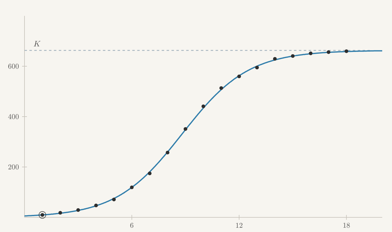
This is worth celebrating! We began with a simple assumption, watched its prediction fail, and used the measurements to suggest a revision. Solving the revised equation then produced a curve that follows the whole experiment.
The logistic model is only a little more complicated than the exponential model: we added one parameter and let the growth per unit of population decrease linearly. Yet that change captures both the early rapid growth and the later slowdown. We have found a model that is still simple enough to understand, but now describes the important behavior over a much longer interval.
We built the logistic model by examining one yeast culture. How much of its success carries over to other populations?
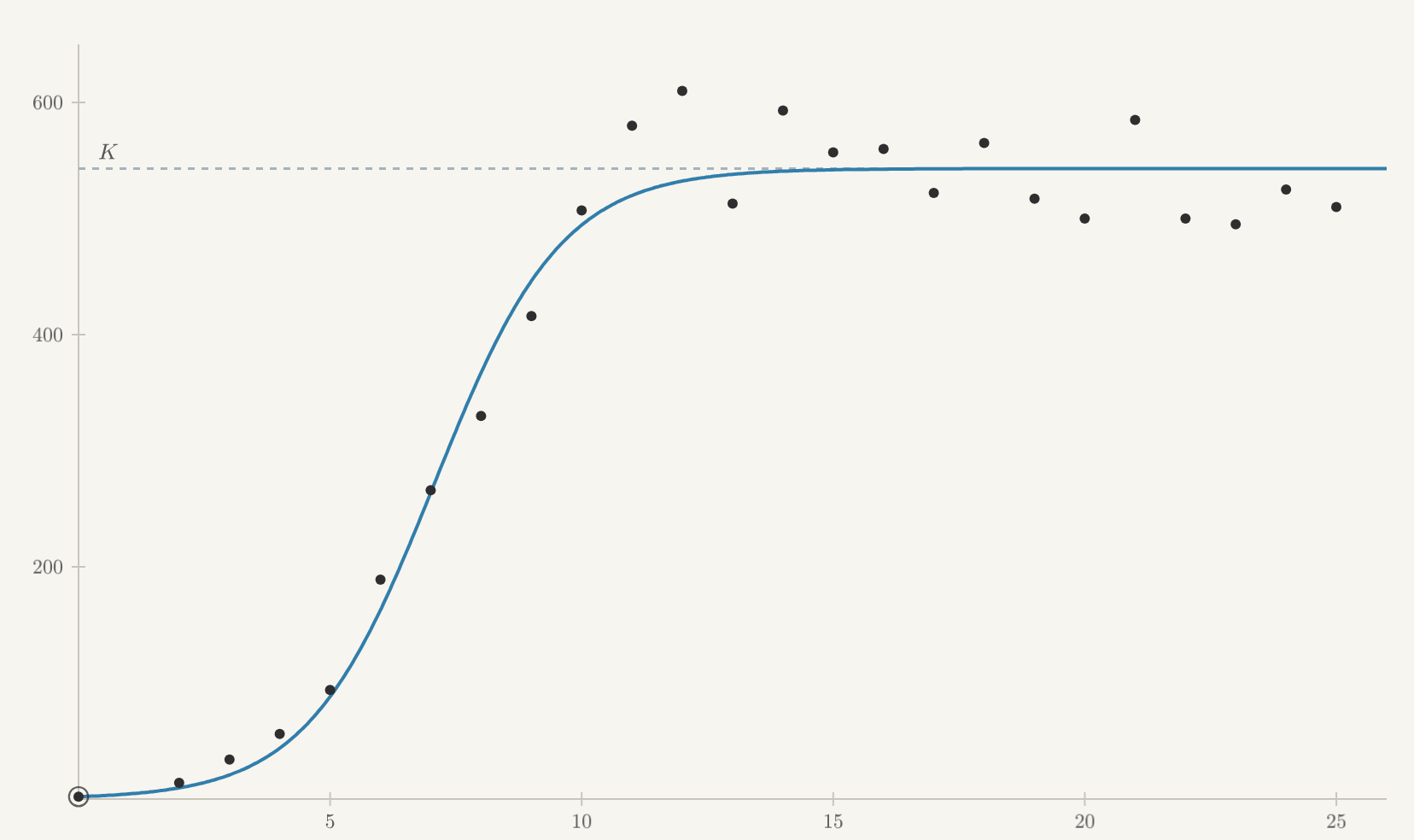
In the 1930s, Georgy Gause measured populations of the single-celled organism Paramecium growing in laboratory cultures. His measurements fluctuate more than Carlson's yeast record, but we can recognize the same broad pattern: rapid growth at first, followed by a slowdown toward a persistent population level.
Try fitting the logistic model to these measurements. We need different
values of
Now make a much larger leap. Instead of a laboratory culture observed over days, consider the population of the United States, recorded by the census every ten years. These measurements span more than two centuries, during which the country's territory, economy, medicine, and ways of life changed enormously. Can the same simple equation describe anything useful here?
The census comparison is striking. A logistic curve captures much of the population's long sweep, despite the enormous complexity of the history behind those measurements. This is the kind of success we are looking for in a simple model: a small amount of mathematics organizes a great deal of observed behavior.
But interpreting its parameters requires judgment. In the laboratory
cultures, the measurements show a recognizable plateau. The census record
has not settled at a population ceiling, so its fitted
And remember our earlier discussion of changing birth rates. The logistic model allows growth per unit of population to change, but it describes that change using only the population itself. A successful fit does not tell us that crowding explains changes in family size, or that immigration and technology can be ignored when predicting the future.
We can learn something from the broad pattern without claiming to have explained every cause. Whether that is enough depends on the question we want the model to answer.
4.2.2Harvesting
So far, we have asked how a population grows. Now suppose we want to use that population: we have a trout pond, and we would like to catch fish. How much can we harvest without eventually emptying the pond?
Let
Fishing introduces another process that changes
For a concrete example, suppose the pond has a carrying capacity of 200 fish and a growth coefficient of 1 per year. Including harvesting gives
where time is measured in years and
The population stays constant when natural growth exactly replaces the fish we catch:
We can find these equilibria graphically. Plot the natural growth rate against the population: it is a parabola. The constant harvesting rate is a horizontal line, and their intersections are the populations where growth and harvesting balance.
Where the parabola lies above the line, the population grows; where it lies below, the population declines. So this one picture also tells us how to draw the phase-line arrows!
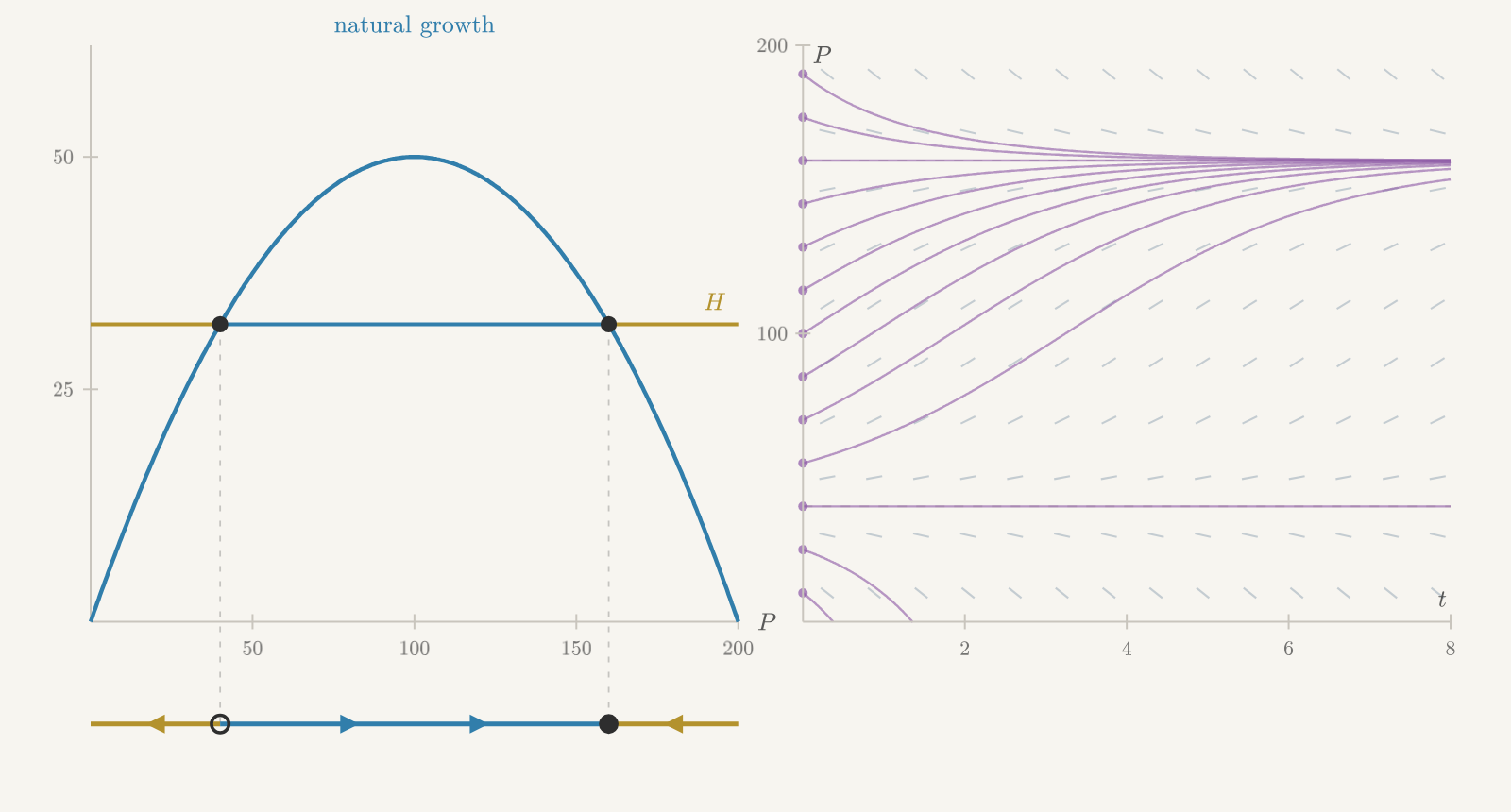
For
If the population falls below
The same harvest can therefore have very different consequences depending on how many fish we begin with!
What happens if we increase the quota? The horizontal line rises, and the
two intersections approach one another. The growth curve reaches its
maximum at
At
A population above
The model has helped us identify a maximum sustainable harvesting rate,
but it has also shown us why operating at that maximum is precarious.
At
There is another limitation we can read directly from the equation.
At
We could instead model harvesting with a term such as
Once again, choosing the term is part of choosing the model. One constant subtraction created a population threshold and changed which long-term outcomes were possible.
4.3Modeling with Systems
So far, we have built models around a single changing quantity: the temperature of an object or the size of a population. But sometimes predicting one quantity requires us to follow another. An object changes the temperature of the room around it, which in turn affects how the object cools. Predators change the population of their prey, while the available prey affects how the predators grow.
In these situations, we need several unknown functions and equations describing how they change together. We are naturally led to a system of differential equations. Let us return to temperature and population to see how this happens.
4.3.1The Coffee and the Room
When we modeled a cooling cup of coffee, we treated the room's temperature as constant. But the hot object also warms its surroundings. What if that change is large enough to matter?
Let
We need a new rule for
The new constant
Putting the two rules together gives our system:
If we set
For
We have not yet developed systematic methods for finding formulas for solutions of systems like this. Learning how to solve and understand systems will be one of the main topics of the rest of the book. But we can already explore them numerically. Euler's method asks us to compute both rates from the current temperatures, then use those rates to advance both temperatures by one short time step. We must compute both rates before updating either temperature, so they refer to the same moment.
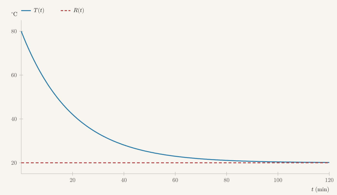
The two temperatures approach agreement. When
Allowing one more quantity to change gave us a different prediction and two equations to study together. Let us now see how interactions between populations lead to the same mathematical need.
4.3.2Interacting Populations
Suppose we want to predict how a population of hares will change. Earlier, we tried to do this using only the number of hares. But if lynx are hunting them, that number alone is no longer enough. The same hare population might grow when there are few lynx and decline when there are many. And the lynx population depends on how much food the hares provide. As with the coffee and the room, predicting either quantity requires us to follow both.
Let
In the absence of lynx, suppose the hares have plenty of food and space. Our earlier assumption of a constant average contribution to net growth gives
We recognize exponential growth. This is our first approximation to what the hares would do without predators.
What should happen to the lynx without hares to eat? We expect their population to decline, but that does not mean every lynx dies at the same instant. For a simple model, suppose that over each short interval, approximately the same fraction of the surviving lynx dies. Twice as many remaining lynx then means twice as many deaths per unit time. This gives
and hence exponential decline,
Now let the two populations interact.
What about encounters? If the populations mix uniformly, doubling the number
of hares should double the opportunities for any lynx to find one, and
doubling the number of lynx should double the total opportunities again. The
simplest expression with both properties is the product
This is the Lotka--Volterra predator--prey model. The coefficients
The limiting cases check the bookkeeping. If
We have built a system because the populations affect one another. A
solution consists of both histories,
We do not need to fit a particular ecosystem in order to explore one
consequence of the model. Choose simple population and time units, take
Here
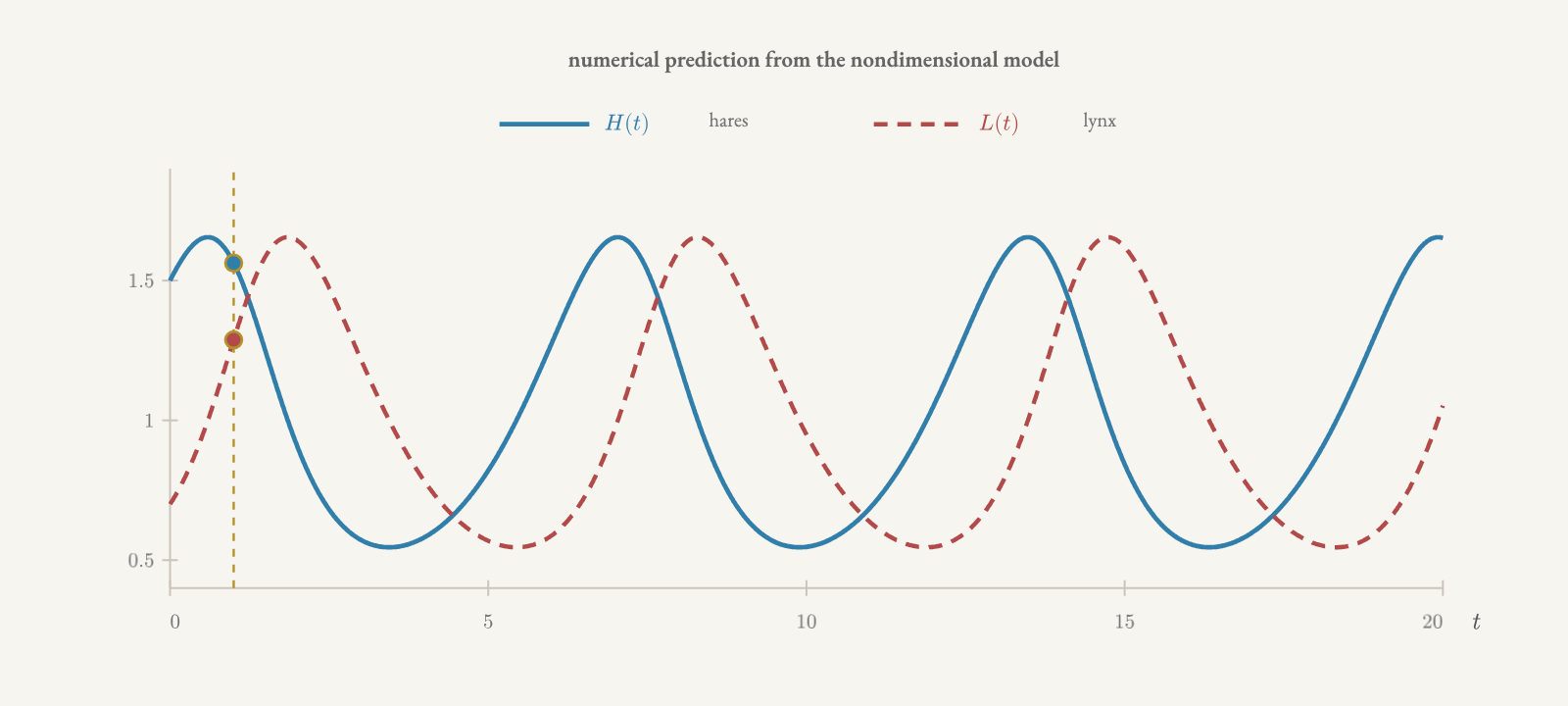
The populations oscillate! When hares are abundant, the lynx have enough food for their population to grow. More lynx then put more pressure on the hares, whose population declines. With less food available, the lynx begin to decline too. Fewer predators give the hares a chance to recover, and the cycle begins again. In the computed histories, the hare peak comes before the lynx peak: food becomes abundant first, and the predator population responds afterward.
Remember the conclusion from chapter 3: a nonconstant solution of a
single smooth autonomous equation
We can explore these oscillations numerically now. Explaining their structure mathematically will be part of our later study of systems.
This is a prediction worth taking back to evidence. The next figure compares the Hudson Bay hare--lynx fur record, a laboratory Paramecium--Didinium experiment, and a prey--predatory-mite experiment. Each population has been divided by its own observed maximum, so we are comparing relative timing, not fitting one scaled model to all three records.
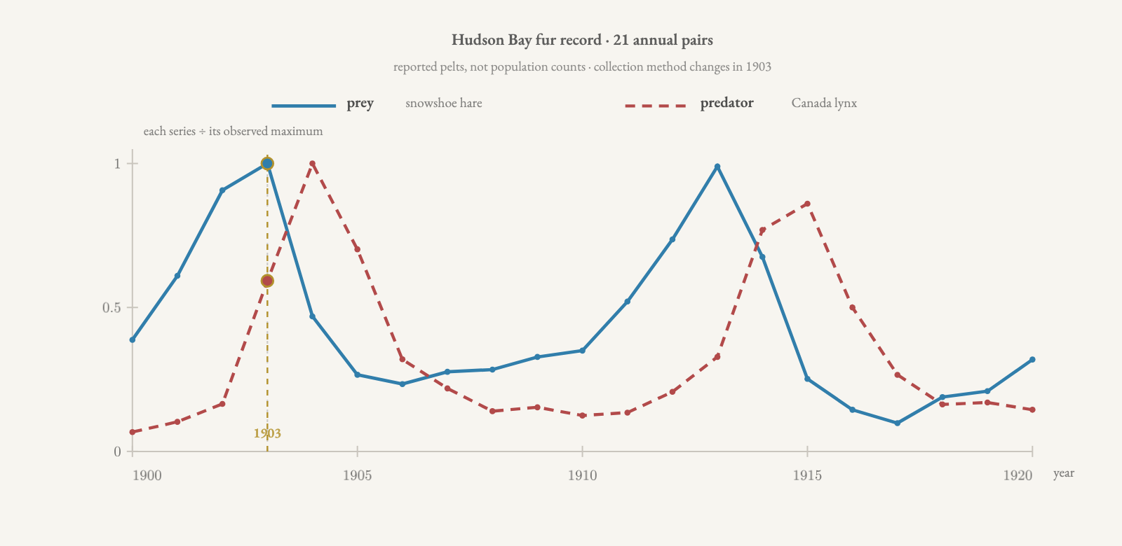
The resemblance is striking. Yet fur returns depend on trapping as well as abundance, and normalization reveals timing while hiding scale. The evidence supports a qualitative mechanism; it does not establish one four-parameter model for every predator--prey system.
In Chapter 3, we sometimes compressed a solution picture onto a phase line by keeping the current value and leaving out time. We can do something similar here, but the current state consists of two populations.
Return to our illustrative model
At any time
Put the hare population on the horizontal axis and the lynx population on the vertical axis. As time passes, this point moves through the plane, tracing a parametric curve. We call this plane the phase plane and the curve a trajectory.
The differential equations tell us how the point moves. Its horizontal
velocity is
Both populations are increasing, so the point moves upward and to the right. We can repeat this calculation at other points to draw a field of arrows.
Our equations are autonomous: their rates depend on the current populations, without explicitly depending on time. This is what lets us assign one fixed arrow to each point in the plane. Whenever the populations have those values, the equations prescribe the same velocity.
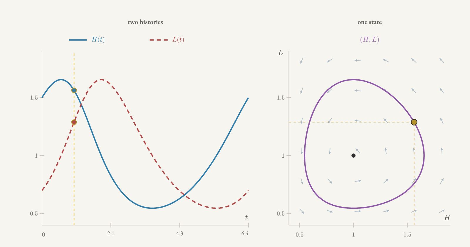
The arrows and trajectories together form a phase portrait. Here the numerical trajectory appears to make a closed loop: the populations return together to their earlier values as the cycle repeats. We have observed this in a computation; we have not yet proved that the trajectory closes.
This curve is not generally the graph of lynx population as a function of hare population. The same number of hares can occur with different numbers of lynx, at different stages of the cycle. Nor does the curve alone tell us when the populations reach a particular point. The time histories retain that information; the phase-plane picture makes their motion together easier to see.
Limited food for the prey
We can now see how each assumption entered the equations: hare reproduction
contributed
Without lynx, our model says the hares grow exponentially forever. But hares need grass and other plants to eat, and the available land cannot support unlimited growth. We have already built a simple model for this kind of limitation! Replace the exponential growth term with logistic growth:
Here
How much difference does this make? If
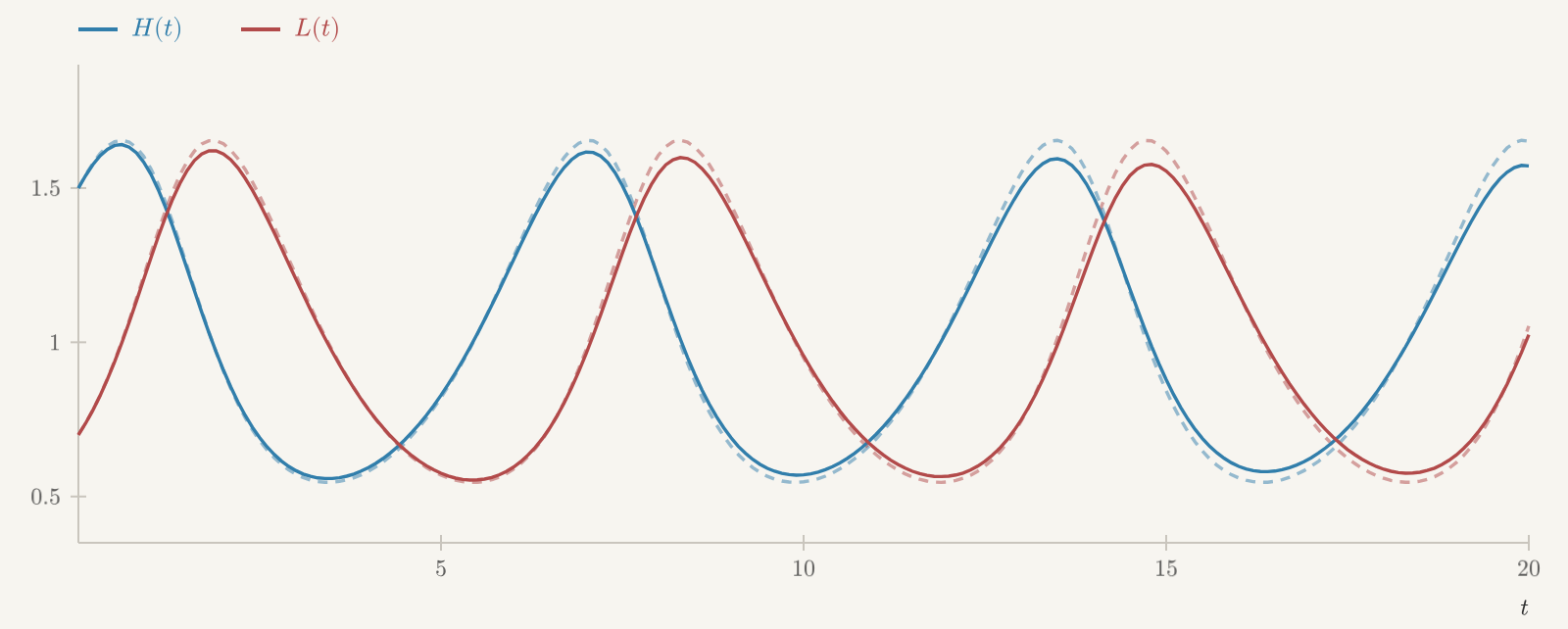
With a large carrying capacity, the hares are far from using up all the grass available to them. Over the first few cycles, the original model does a pretty good job! The extra term makes little difference to the behavior we see. For smaller carrying capacities, the peaks in the revised model visibly shrink as time passes. The cycles no longer repeat in the same way.
Let us follow that change in the phase plane. A repeating population cycle would trace the same closed loop each time. What happens to the trajectory when the successive peaks get smaller?
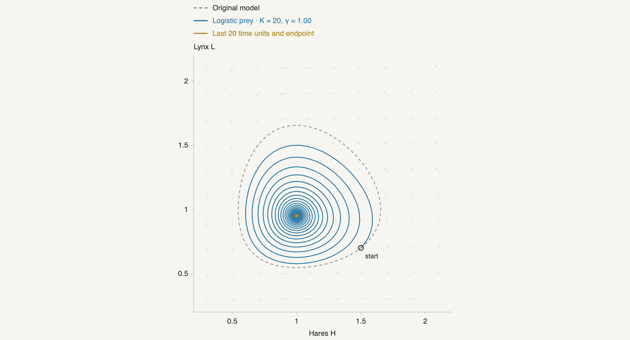
The trajectory winds inward: each trip around the center corresponds to
a smaller swing in the populations. The computation suggests that both
populations eventually settle at constant values. Try increasing
We did not need to account for grass to explain why predators and prey can oscillate. But including it changes our prediction about whether those oscillations persist. If food is plentiful and we want to follow just a few cycles, the simpler model may be enough. If we want to predict what happens over many cycles, even a small limitation on the hares' food supply can matter. How far ahead we want to predict is part of choosing the model!
Hunting interacting populations
For our second extension, return to the original predator–prey model and
add hunting. The trout pond taught us that a harvesting term is a modeling
decision, and that removing a fixed fraction of the population is the
policy which shuts itself off as the
population disappears. So suppose hunters remove hares at a per-capita rate
Before computing anything, guess. Hunting hares should mean fewer hares, and
hunting lynx should mean fewer lynx. Now look for the balance point, the
state at which neither population changes. When both populations are positive,
the hare rate vanishes only when
Read this carefully, because it contradicts the guess. The hare balance depends only on how hard we hunt lynx, and the lynx balance depends only on how hard we hunt hares. Hunting hares leaves the hare balance exactly where it was and lowers the lynx balance instead.
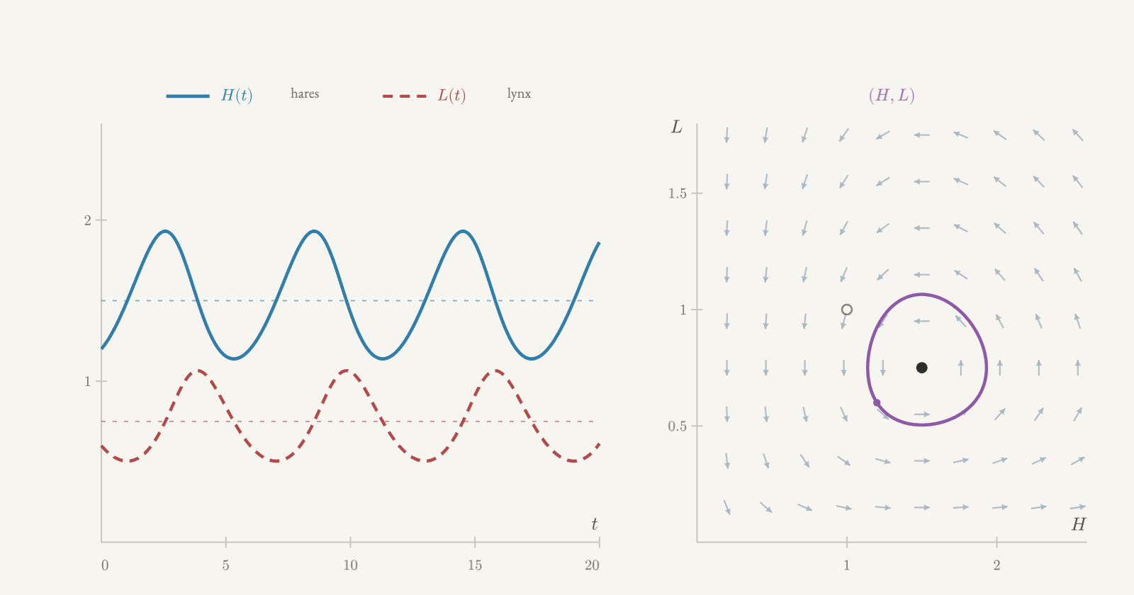
The figure shows why the guess was wrong. Hunting hares does remove hares,
but every hare we take is one the lynx do not eat. The hares can only hold
their own once the lynx have declined to
Nothing about the individual terms announced this. The term
Learning rates from an outbreak
An epidemic gives us another reason to follow several populations. The
number of infectious people matters, but it is not enough: the same number
can spread an illness very differently depending on how many people are
still able to catch it. Let
How quickly do new infections occur? We can reuse our reasoning about
predator--prey encounters. If people mix uniformly, doubling the susceptible
population should double an infectious person's opportunities to pass on
the illness. Doubling the infectious population should double the total
opportunities again. This suggests an infection rate
For recovery, suppose approximately the same fraction of the infectious
population recovers over each short interval of a given length. Twice as many
infectious people then means twice as many recoveries per unit time, giving
a recovery rate
Now follow where people go. Each new infection removes one person from
These are the SIR equations. The same
As with the cooling constant, our assumptions have given us a model without
determining its constants. We can learn about
In October 1967, a common-cold outbreak on Tristan da Cunha was recorded
through daily reports of illness and recovery. A published
table of 21 daily observations
gives us two curves to compare with our model. We use the number currently
ill as an approximation to
There is another unknown here: how many people were susceptible at the
start? We must estimate
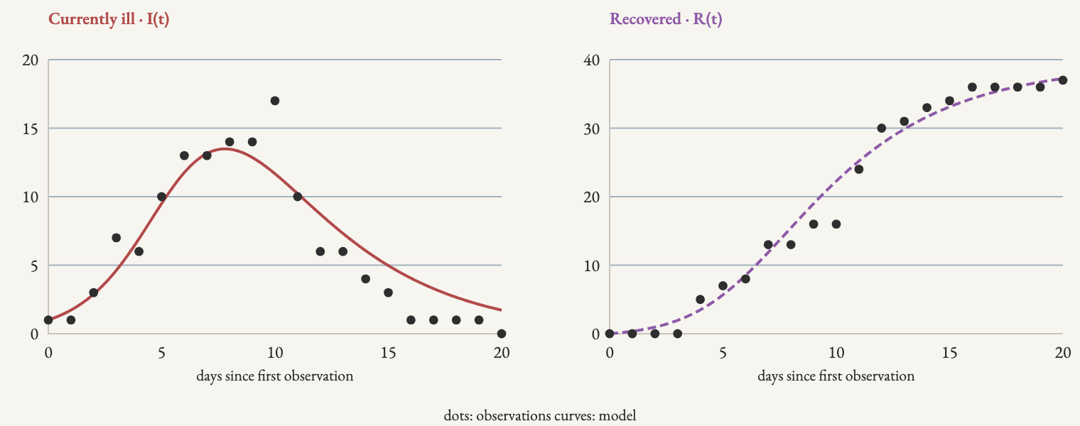
The model captures the rise and fall of illness along with the accumulating
recoveries. Try changing one parameter at a time. Increasing
The equations can also suggest a more direct way to estimate a constant.
In the exercises, we use
There is still room to improve the model. The fit misses the sharp illness peak and predicts a slower decline. Its estimate of about forty initially susceptible people is also much smaller than the island's population: the fit does not tell us whether the others were immune or whether uniform mixing was a poor assumption. These are estimates within our model, not direct measurements of its mechanisms.
We could revise those assumptions too. An SEIR model adds an exposed group between susceptible and infectious, allowing time between catching an illness and being able to transmit it. The published comparison considers this extension using the same data.
From the coffee and the room to interacting populations, the need for systems has come from asking what else we must keep track of. Once those quantities affect one another, their equations belong together. We can already compute approximate solutions and compare them with observations; learning how to solve and understand these systems will be one of the main tasks of the rest of the book.
4.4Forces and Second-Order Equations
Pull a mass attached to a horizontal spring away from its resting position and let go. It moves back and forth. How could we build a model of that motion?
Let
4.4.1From a restoring force to an equation
The spring pulls the mass back toward its resting position. When
The constant
What does this force tell us about
Our description has led us to a second-order differential equation! The force gives us a rule for the second derivative. In particular, a mass to the right of its resting position has negative acceleration. It might still be moving right, but the spring is slowing that motion and will pull it back. The same position can occur on the outward trip and on the return trip, with different velocities.
This is why knowing the initial position alone cannot determine the motion. We must also specify how we launch the mass:
These are our two initial conditions. As with interacting populations, we have found that predicting one quantity requires more information than its current value.
4.4.2What motion does the model predict?
Dividing by
so choosing
satisfies both the equation and our initial conditions: at
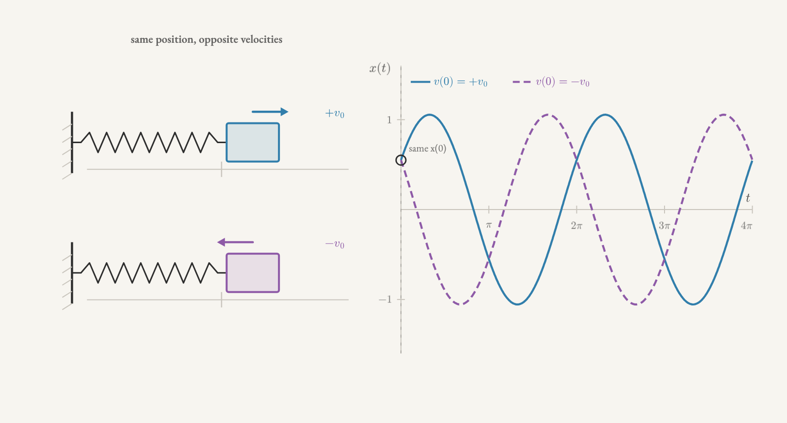
The model predicts oscillation. For a nonzero motion, the time to complete one cycle is
A heavier mass oscillates more slowly; a stiffer spring makes it oscillate
more quickly. We can also work backward: measuring the period for a known
mass lets us determine
4.4.3Revising the model: resistance to motion
Our formula predicts that the oscillations continue forever, with the same amplitude. A spring we release on a table usually settles down. What did we leave out? We deliberately ignored resistance to motion. Let us revisit that choice.
A resisting force should point opposite the velocity: left when the mass
moves right, and right when it moves left. For a simple model, suppose its
magnitude is proportional to speed. With a new positive constant
Notice the difference between the two forces. The spring responds to position; drag responds to velocity. They can point in the same direction or in opposite directions, depending on how the mass is moving. Adding their contributions to the total force gives
We have changed the model by adding one term. Setting
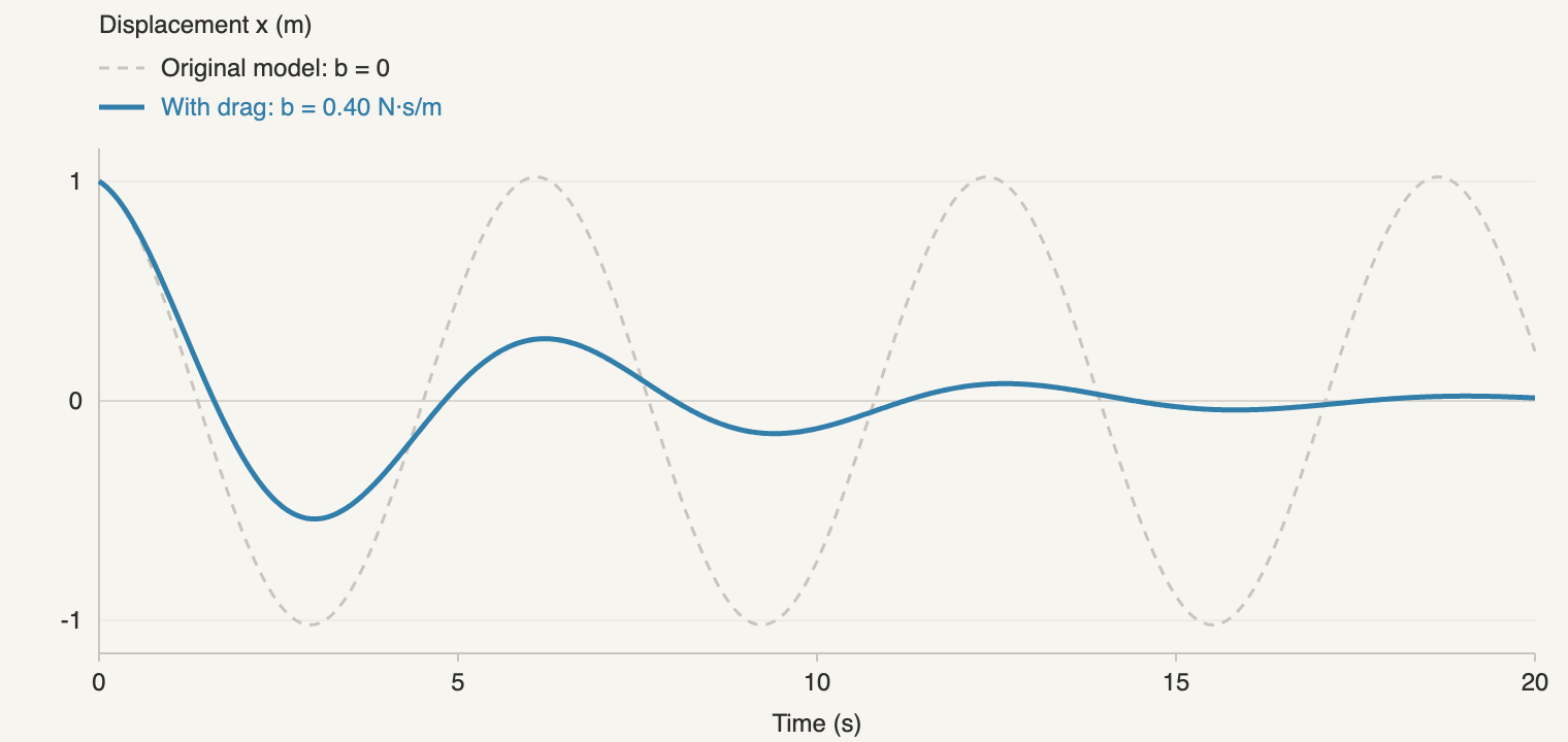
With these positive choices of
How can we compute these motions with the first-order methods we already
know? Let
The first equation says how velocity changes position; the second says
how the forces change velocity. Starting from
Position and velocity together form the state of this model. We can describe its motion with one second-order equation or two first-order equations. So the two extensions we have met in this chapter are connected: learning to work with systems will also help us understand equations with higher derivatives.
4.5Appendix: Modeling Earth's Temperature
Sunlight warms Earth, while radiation carries energy away into space. Can we turn this description into a model of Earth's temperature? Let us try the same process we used for coffee and populations: choose what to hold constant, build an equation, and see what its predictions tell us.
4.5.1A planet with one temperature
Our ingredients are the surface temperature, the sunlight Earth absorbs,
and the radiation it emits. Let
How should these quantities determine
To make this precise, suppose a fixed amount of energy is needed to raise
the temperature by one degree. Call that amount
We need a rule for the outgoing radiation. Here physics supplies one:
an ideal emitter, called a blackbody, radiates at rate
We now have a model! The temperature varies, while
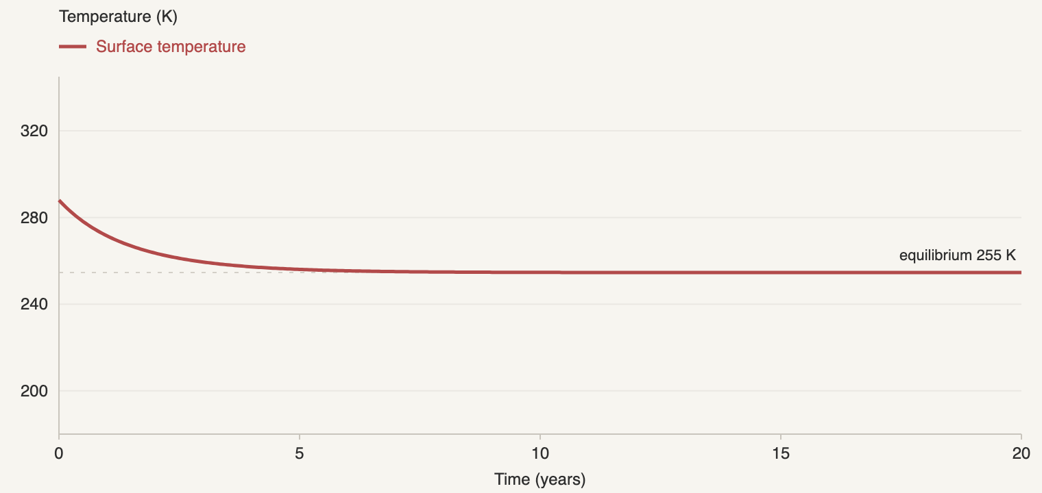
At a constant temperature,
Above this temperature, radiation removes more energy than sunlight
supplies, so the planet cools; below it, the planet warms. That explains
where the plotted solutions are heading. Changing
The prediction is about
4.5.2Adding an atmosphere
We let radiation escape straight from the surface to space. But Earth's atmosphere absorbs some of that radiation and emits radiation of its own, including radiation back toward the surface. To include this interaction, we need to follow the atmosphere's temperature too, just as we followed both the coffee and the room.
Call the surface temperature
Sunlight is concentrated at shorter wavelengths than the radiation emitted
by Earth's surface, and the atmosphere absorbs them differently. For a
simple model, suppose sunlight passes through the atmosphere and warms
the surface, while all infrared radiation from the surface is absorbed
by the atmosphere. Keep the same absorbed sunlight rate
Absorbing radiation warms the atmosphere. The atmosphere also emits
radiation of its own: downward toward the surface and upward toward space.
Let us apply the same blackbody law to each side of our layer, giving an
emission rate
We can now write the surface's equation. It gains energy from sunlight
at rate
The atmosphere gains energy from the surface at rate
The factor of two counts the two directions. Each temperature now affects the other's rate of change, giving us a system. Choosing both initial temperatures lets us explore it numerically as we did with the coffee and the room.
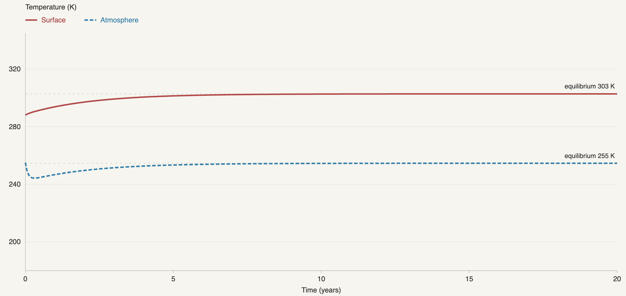
The temperatures settle at different values. Setting both derivatives to zero tells us that incoming and outgoing radiation balance for each:
Substituting the second equation into the first gives
Adding the atmosphere has made the surface warmer: it now receives radiation from the atmosphere as well as sunlight. Unlike the coffee and room, these temperatures need not become equal, because energy keeps entering from the Sun and leaving for space. This simple greenhouse model shows how an atmosphere can maintain a warmer surface.
But
We have repeated the same process: a choice of quantities and simple rules gave us an equation; its prediction led us to revise those choices. Adding a second temperature captured an important interaction, and the new prediction suggests where to look next.
Further Reading
Raymond Pearl's 1927 survey, “The Growth of Populations”, reprints Carlson's yeast measurements and places the logistic model in its early historical setting.
Georgy Gause's 1934 book The Struggle for Existence reports the Paramecium cultures used in the logistic data laboratory.
The U.S. Census Bureau's historical population tables provide the decennial counts used there from 1790 through 2020.
Thomas W. Judson's open ODE Project develops population, harvesting, predator--prey, epidemic, and mechanical models through activities and computation.
Brian Rose's open, notebook-based Climate Laboratory Book builds energy- balance and greenhouse models in more physical detail than we used here.
Courchamp, Clutton-Brock, and Grenfell's review “Inverse Density Dependence and the Allee Effect” explains the biological mechanisms behind low-population decline and the strong-Allee model.
Problems
Modeling begins before an equation is solved. In every problem, name the state, say what each term means, and check signs or units before trusting a calculation. The explorations ask you to make new modeling choices; more than one answer may be defensible when the assumptions are stated clearly.
Check Your Understanding
1Read the assumptions from the equation
For each model, identify the state variables and parameters, describe the mechanism represented by every term, and give one limiting case which checks your interpretation.
2Predicting the coffee's temperature
A cup of coffee sits in a room held at
Use the two measurements to determine
Predict the coffee's temperature twenty minutes after the first measurement.
3Exponential first, logistic later
A bacterial culture begins with mass
Write the exponential model and predict the mass after six hours.
Suppose the environment has carrying capacity
At what population does the logistic model's total growth rate reach its maximum? At what population has its per-capita rate fallen to half of the low-density value? Explain why these are the same population in this model.
4Harvesting a pond
For
Complete the square in the natural-growth term to show that its maximum is
For
A manager wants an attracting equilibrium of at least
5A tank as a balance law
A tank initially holds
Derive the differential equation and check the units of both terms.
Find and classify the equilibrium volume without solving the equation.
Solve the initial value problem. Use the formula to answer when the volume is
within
The physical tank holds only
6What changes a climate equilibrium?
The absorbed sunlight in the climate appendix can be written as
Suppose absorbed sunlight increases by a constant amount
Derive the equilibrium temperature and show directly which parameters can move it.
Without solving for
Compute the new equilibrium when
7Two histories, one moving point
Consider the chapter's predator–prey model with
Calculate
Draw the four points in the phase plane and attach an arrow showing the velocity at each. Interpret each arrow in terms of growing or declining populations.
In the chapter's figure showing time histories beside the phase-plane trajectory, locate a maximum of the hare population and the next maximum of the lynx population. Mark the corresponding points on a sketch of the trajectory. At which point is the motion vertical, and at which is it horizontal? Explain using the derivatives.
At the states
8Transfers must cancel
Here we use fractions of the population rather than counts. If the constant
total population is
A quantity computed from a solution is conserved if it remains constant along that solution.
Differentiate
Explain why knowing
At the state
Perform one simultaneous Euler step with
Add the three Euler update formulas at an arbitrary state. Show that their sum is unchanged by every simultaneous step, apart from rounding errors in a computer calculation.
A student updates
9Spring data determine parameters
A
Use
The mass begins
Find the first time at which the mass passes through equilibrium. Check that the sign of its velocity then agrees with the initial motion.
Let
Explorations
10A threshold built one factor at a time
Suppose a population has trouble finding mates when its numbers are small.
We want a model in which populations below
Draw the desired phase line. Where must the rate vanish?
Start with the logistic rate
Find a dimensionless factor, linear in
Describe the futures of populations starting at
If time is measured in years, what units must
11Constant harvest or proportional harvest?
Replace the fixed quota in the trout model by removal proportional to the
population:
Find and classify the equilibria as
Compare the behavior near
Compare the constant quota
12The vanishing snowball
A spherical snowball melts at a rate proportional to its surface area. Its
radius is
Start with volume
Determine when the snowball disappears. Why is the radius linear in time even though both volume and area are nonlinear functions of radius?
Name one physical change near the end of melting which could make the model fail.
13An oven that is still warming
An object is placed in an oven just as the oven is switched on. Both
initially have temperature
where time is measured in minutes and temperature in degrees Celsius. Model
the object by a single temperature
Write the initial value problem for
In Chapter 2 we subtracted the constant surrounding temperature. Try the
corresponding substitution
What does the extra term represent?
Solve for
Show that
The temperature difference
14A partially transparent greenhouse
Modify the climate appendix's greenhouse model by assuming the atmosphere absorbs a
fraction
Let
Write differential equations for
Add the equations to find
Identify the two ways radiation escapes to space. Explain why energy exchanged between the surface and atmosphere disappears from this combined balance.
Suppose
Now set
Find the value of
15Vaccination as a transfer
Suppose susceptible individuals in an SIR model are vaccinated at a
per-capita rate
Modify all three equations. Make the new transfer appear once with a minus sign and once with a plus sign.
Show that
At what instantaneous rate does vaccination reduce the susceptible
population when
Python: Models as Experiments
16Recover a growth law from Carlson's data
The arrays below contain the eighteen hourly yeast measurements used in the chapter.
import numpy as np
import matplotlib.pyplot as plt

t = np.arange(1, 19, dtype=float)
N = np.array([
    9.6, 18.3, 29.0, 47.2, 71.1, 119.1, 174.6, 257.3, 350.7,
    441.0, 513.3, 559.7, 594.8, 629.4, 640.8, 651.1, 655.9, 659.6
])Compute the midpoint population and midpoint estimate of per-capita growth for every consecutive pair. Plot the estimated rate against the midpoint population. Label the axes with units.
Use np.polyfit to fit a line to this rate plot. Read estimates of
Plot the data together with the logistic solution using your estimates. Describe one feature the curve captures and one feature the two-parameter model leaves unexplained.
17Force a climate model
Suppose the absorbed sunlight in the climate appendix changes by a
prescribed amount
Adapt your Euler function from Chapter 2 to the model
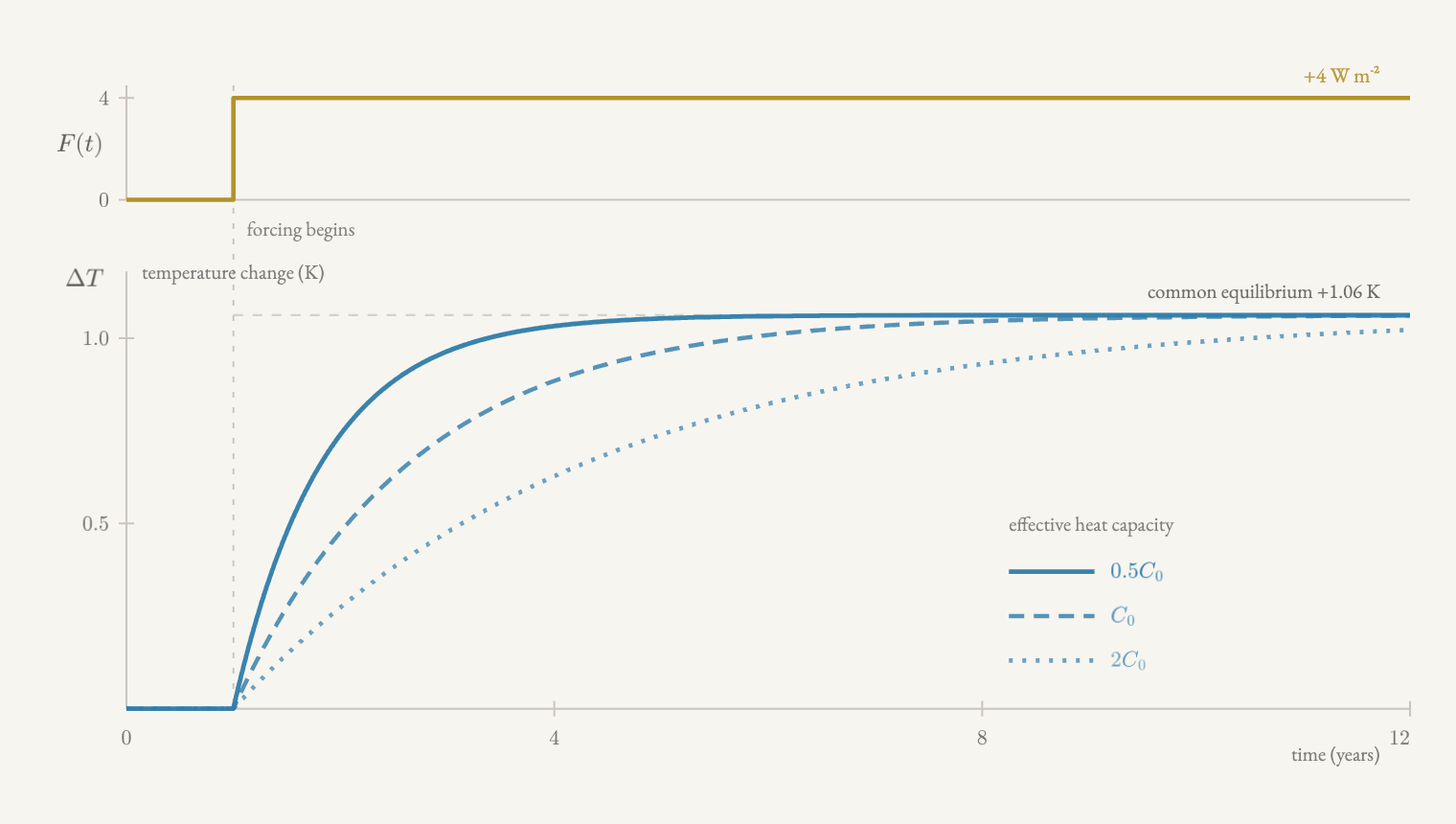
Use
Write three forcing functions: a step from
Plot the response to each forcing for two values of
For the periodic forcing, measure the time difference between one forcing
peak and the following temperature peak. How does this lag change with
18Does one recovery rate describe the outbreak?
These are the daily illness and recovery counts from the Tristan da Cunha
record used in the chapter. Time is measured in days from the first
observation. As in the text, use the number currently ill as an approximation
to the infectious population
I = [1,1,3,7,6,10,13,13,14,14,17,10,6,6,4,3,1,1,1,1,0]
R = [0,0,0,0,5,7,8,13,13,16,16,24,30,31,33,34,36,36,36,36,37]Starting from
on any interval with a nonzero denominator. Check the units.
Estimate the integral over
Repeat the calculation separately for
Use your whole-record estimate
Plot these reconstructed recovery counts alongside the observations. Why must the final counts agree? Do the intermediate counts agree?
Discuss what this comparison tells us about using one constant recovery rate. Consider the discrete observations, the integral approximation, and the assumption that being ill coincides with being infectious. Does disagreement by itself establish that the biological recovery rate changed?
19Simulate transfers and audit conservation
Write a function returning the three SIR rates and use simultaneous vector Euler updates
state = state + h * rates(state)to simulate an epidemic from
Plot all three compartments against time and plot S + I + R on a second
axis. Report the largest deviation of the total from
Add the vaccination transfer from the previous exploration. Compare the
peak infected fraction and the time of that peak for
Deliberately implement the sequential-update mistake from the routine problem. Plot the total again. Explain how a conservation law became a test of your code rather than merely a fact about the equations.