Chapter 3

A Glimpse of the Theory

There is an old joke that a mathematician will prove a problem has a solution, then stop and leave finding it to the engineers. There is some truth to this! Knowing that a solution exists can be the beginning of a mathematical investigation, even if we never write it down.

Suppose we are studying a differential equation and want to say, “Take the solution $𝑦 (𝑡)$ , and now let us see what we can learn about it.” Perhaps we want to know whether it stays positive, whether it can pass another solution, or whether it must keep increasing. We might be able to answer these questions directly from the equation. But are we entitled to begin with “take the solution”? Is there a function there to investigate? And does calling it the solution make sense?

We might not even know the exact equation. A model could contain parameters we have not measured precisely, or a function whose general properties we understand without knowing its formula. Can we make statements which hold for every equation consistent with that information?

These are questions for a general theory of differential equations. We want results whose hypotheses describe what we need to know about an equation, and whose conclusions tell us something about its solutions. Such results let us reason about functions we have not found, and about whole classes of equations at once.

We will begin by establishing existence: that there is a solution to investigate. We will also ask about uniqueness: whether two solutions satisfying the same equation and initial condition must agree. For one important class of equations, the calculus from the last chapter is already enough to prove both.

3.1Existence and Uniqueness for Linear Equations

We have already proved our first existence-and-uniqueness result, although we were thinking about antidifferentiation when we did it. Suppose $𝑓$ is continuous on an open interval $𝐼$ containing $𝑡 0$ . Then

𝑦' = 𝑓 (𝑡), 𝑦 (𝑡 0) = 𝑦 0

has the solution

𝑦 (𝑡) = 𝑦 0 + \int 𝑡 𝑡 0 𝑓 (𝑠) 𝑑 𝑠 .

The Fundamental Theorem of Calculus verifies that its derivative is $𝑓 (𝑡)$ , and setting $𝑡 = 𝑡 0$ gives the required initial value. We have produced a solution, so we have proved existence.

But we also proved uniqueness. Suppose someone proposes another solution. Whatever function they give us, the Fundamental Theorem of Calculus requires it to satisfy

𝑦 (𝑡) - 𝑦 0 = \int 𝑡 𝑡 0 𝑦' (𝑠) 𝑑 𝑠 = \int 𝑡 𝑡 0 𝑓 (𝑠) 𝑑 𝑠 .

That forces exactly the formula above. There is no room for a different answer!

Notice how little we needed to know about $𝑓$ . We never chose a particular function, and we never evaluated an integral. Continuity was enough to make the construction work. Moreover, it works throughout $𝐼$ : for every $𝑡$ in that interval, we can integrate along the segment joining $𝑡 0$ to $𝑡$ .

Now let us change the equation a little:

𝑦' = 𝑓 (𝑡) 𝑦, 𝑦 (𝑡 0) = 𝑦 0 .

The rate now depends on the unknown value as well as on time, but separation gives us a way forward. On an interval where $𝑦 \neq 0$ ,

𝑑 𝑦 𝑦 = 𝑓 (𝑡) 𝑑 𝑡 .

To keep the notation manageable, write

𝐴 (𝑡) = \int 𝑡 𝑡 0 𝑓 (𝑠) 𝑑 𝑠 .

Thus $𝐴' = 𝑓$ and $𝐴 (𝑡 0) = 0$ . Integrating the separated equation gives

l n | 𝑦 | = 𝐴 (𝑡) + 𝐶,

and exponentiating produces a family of the form $𝑦 = 𝐶 𝑒 𝐴 (𝑡)$ , with a renamed constant. Allowing $𝐶 = 0$ includes the constant solution we excluded when dividing. The initial condition selects $𝐶 = 𝑦 0$ , suggesting

𝑦 (𝑡) = 𝑦 0 𝑒 𝐴 (𝑡) .

Let us check it:

𝑦' (𝑡) = 𝑦 0 𝑒 𝐴 (𝑡) 𝐴' (𝑡) = 𝑓 (𝑡) 𝑦 (𝑡), 𝑦 (𝑡 0) = 𝑦 0 𝑒 0 = 𝑦 0 .

The formula works for every initial value, including zero, and it is defined throughout $𝐼$ . We have proved existence again.

Have we also proved uniqueness? Our separation calculation divided by $𝑦$ , so we need to be careful about what happens at zero. It is easy to verify that the zero function solves the equation. What we need to rule out is some other function which satisfies the same initial condition but behaves differently afterward.

The formula we found suggests how to proceed. If $𝑦 = 𝐶 𝑒 𝐴 (𝑡)$ , then multiplying by $𝑒 - 𝐴 (𝑡)$ leaves a constant. Could the equation itself force that product to be constant?

Take any solution of $𝑦' = 𝑓 (𝑡) 𝑦$ . By the product rule,

𝑑 𝑑 𝑡 (𝑒 - 𝐴 (𝑡) 𝑦 (𝑡)) = 𝑒 - 𝐴 (𝑡) 𝑦' (𝑡) - 𝐴' (𝑡) 𝑒 - 𝐴 (𝑡) 𝑦 (𝑡) = 𝑒 - 𝐴 (𝑡) (𝑦' (𝑡) - 𝑓 (𝑡) 𝑦 (𝑡)) = 0 .

A function with derivative zero on an interval is constant, by the Mean Value Theorem. At the initial time, this constant is

𝑒 - 𝐴 (𝑡 0) 𝑦 (𝑡 0) = 𝑦 0 .

Therefore every solution with the prescribed initial value must satisfy

𝑒 - 𝐴 (𝑡) 𝑦 (𝑡) = 𝑦 0,

which forces $𝑦 (𝑡) = 𝑦 0 𝑒 𝐴 (𝑡)$ .

This argument never divided by $𝑦$ , so it works even when $𝑦 0 = 0$ . We have proved uniqueness for every initial value.

The factor $𝑒 - 𝐴 (𝑡)$ is an integrating factor, just like the one we constructed in the last chapter. Here it turned the equation into the assertion that a product has derivative zero. Let us see what happens if we change the equation once more:

𝑦' = 𝑓 (𝑡) 𝑦 + 𝑔 (𝑡) .

An equation of this form is called a first-order linear equation. We now have a prescribed contribution $𝑔 (𝑡)$ to the rate, in addition to the term proportional to $𝑦$ . The same product-rule calculation gives

𝑑 𝑑 𝑡 (𝑒 - 𝐴 (𝑡) 𝑦 (𝑡)) = 𝑒 - 𝐴 (𝑡) (𝑦' (𝑡) - 𝑓 (𝑡) 𝑦 (𝑡)) = 𝑒 - 𝐴 (𝑡) 𝑔 (𝑡) .

The product is no longer constant, but its derivative is a known function of time. We are back to the first problem we solved: accumulating a prescribed rate.

This gives us a theorem for the entire class.

Theorem 3.1 (Existence and uniqueness for first-order linear equations). Let $𝑓$ and $𝑔$ be continuous on an open interval $𝐼$ , and let $𝑡 0 \in 𝐼$ . Then, for every initial value $𝑦 0$ , the initial value problem

𝑦' = 𝑓 (𝑡) 𝑦 + 𝑔 (𝑡), 𝑦 (𝑡 0) = 𝑦 0

has exactly one solution on all of $𝐼$ .

Proof. Keep

𝐴 (𝑡) = \int 𝑡 𝑡 0 𝑓 (𝑠) 𝑑 𝑠 .

The product derivative we just found tells us to integrate:

𝑒 - 𝐴 (𝑡) 𝑦 (𝑡) - 𝑒 - 𝐴 (𝑡 0) 𝑦 (𝑡 0) = \int 𝑡 𝑡 0 𝑒 - 𝐴 (𝑠) 𝑔 (𝑠) 𝑑 𝑠 .

Since $𝐴 (𝑡 0) = 0$ and $𝑦 (𝑡 0) = 𝑦 0$ , we obtain the candidate

𝑦 (𝑡) = 𝑒 𝐴 (𝑡) (𝑦 0 + \int 𝑡 𝑡 0 𝑒 - 𝐴 (𝑠) 𝑔 (𝑠) 𝑑 𝑠) .

Every part of this expression is defined for every $𝑡 \in 𝐼$ . Continuity of $𝑓$ gives us $𝐴$ , and continuity of $𝑒 - 𝐴 𝑔$ gives us the second integral. To verify the equation, differentiate using the product rule and the Fundamental Theorem of Calculus:

𝑦' (𝑡) = 𝑓 (𝑡) 𝑒 𝐴 (𝑡) (𝑦 0 + \int 𝑡 𝑡 0 𝑒 - 𝐴 (𝑠) 𝑔 (𝑠) 𝑑 𝑠) + 𝑒 𝐴 (𝑡) 𝑒 - 𝐴 (𝑡) 𝑔 (𝑡) = 𝑓 (𝑡) 𝑦 (𝑡) + 𝑔 (𝑡) .

At $𝑡 = 𝑡 0$ , the integral vanishes and the exponential equals $1$ , so $𝑦 (𝑡 0) = 𝑦 0$ . This proves existence on all of $𝐼$ .

For uniqueness, suppose $𝑦 1$ and $𝑦 2$ both solve the initial value problem. We want to show that they agree, so let us study their difference:

𝑢 = 𝑦 2 - 𝑦 1 .

Subtracting the equations gives

𝑢' = (𝑓 (𝑡) 𝑦 2 + 𝑔 (𝑡)) - (𝑓 (𝑡) 𝑦 1 + 𝑔 (𝑡)) = 𝑓 (𝑡) 𝑢 .

Their initial values agree, so $𝑢 (𝑡 0) = 0$ . But we have already proved that $𝑢' = 𝑓 (𝑡) 𝑢$ with this initial value has exactly one solution: $𝑢 = 0$ . Consequently $𝑦 1 = 𝑦 2$ , proving uniqueness. ∎

This is a big deal. Whenever we have a first-order linear equation with continuous coefficients and an initial value, we are entitled to say “take the solution” and begin investigating it. The theorem guarantees that there is a function there, that the initial value selects it uniquely, and that it exists throughout the coefficient interval. If the coefficients are continuous for all real time, the solution exists for all real time too.

The result applies even when we have not specified the coefficients completely. We might know their signs, bounds on their values, or how they depend on a parameter. As long as they are continuous, existence and uniqueness are settled. Those other properties can then become the information we use to investigate the solution.

And uniqueness tells us what a successful guess has accomplished. If we find a function satisfying the equation and initial condition, it must agree with the solution constructed in the proof. As we vary $𝑦 0$ , the formula gives every solution on $𝐼$ , because every such solution has a value at $𝑡 0$ .

Of course, the formula may be an inconvenient way to compute. It contains an integral inside an exponential, and then another integral involving that exponential. Euler's method gives us a different way to approximate values. But the formula has already done its theoretical work: we know that the solution exists and is unique without evaluating either integral.

We have another calculus technique available. Separation of variables also produced answers in the last chapter, including for nonlinear equations. Can we use it to establish a general result too? And will its construction work throughout the interval where the equation is defined?

3.2Existence and Uniqueness for Separable Equations

In the last chapter, separation turned an equation of the form

𝑦' = 𝑔 (𝑡) ℎ (𝑦)

into two integration problems. But the resulting relationship did not always give us an explicit formula for $𝑦$ . Sometimes there was more algebra to do, and sometimes we left the answer implicit. Can we still use that relationship to prove that a solution exists and is unique? And how far in time can we follow it?

Suppose $𝑔$ is continuous on an open interval of times $𝐼$ , and $ℎ$ is continuous on an open interval of possible values of $𝑦$ . Choose an initial time $𝑡 0$ and an initial value $𝑦 0$ in these intervals. For now, assume $ℎ (𝑦 0) \neq 0$ , so we do not begin at one of the equilibrium solutions that division would discard.

Recall what separation tells us to try:

\int 𝑦 (𝑡) 𝑦 0 𝑑 𝑢 ℎ (𝑢) = \int 𝑡 𝑡 0 𝑔 (𝑠) 𝑑 𝑠 .

Each side integrates a known function; the unknown value $𝑦 (𝑡)$ appears as the upper limit on the left. Let us name the two functions defined by these integrals:

𝐻 (𝑦) = \int 𝑦 𝑦 0 𝑑 𝑢 ℎ (𝑢), 𝐺 (𝑡) = \int 𝑡 𝑡 0 𝑔 (𝑠) 𝑑 𝑠 .

The relationship becomes $𝐻 (𝑦 (𝑡)) = 𝐺 (𝑡)$ . If we can invert $𝐻$ , we can recover the unknown function:

𝑦 (𝑡) = 𝐻 - 1 (𝐺 (𝑡)) .

Does $𝐻$ have an inverse? Since $ℎ$ is continuous and $ℎ (𝑦 0) \neq 0$ , there is a small open interval $𝐽$ around $𝑦 0$ on which $ℎ$ never vanishes. It cannot change sign there without passing through zero. The Fundamental Theorem of Calculus gives

𝐻' (𝑦) = 1 ℎ (𝑦),

so $𝐻'$ also has a constant, nonzero sign on $𝐽$ . Thus $𝐻$ is strictly monotone and has an inverse on its range. The inverse-function rule from calculus tells us that this inverse is differentiable.

We do not have to find a formula for the inverse to know that it exists! Monotonicity has established that each value in the range of $𝐻$ comes from exactly one value of $𝑦$ .

There is one more thing to check: does $𝐺 (𝑡)$ belong to that range? At the initial time,

𝐺 (𝑡 0) = 0 = 𝐻 (𝑦 0) .

Since $𝑦 0$ is inside $𝐽$ , the range of $𝐻$ contains an open interval around zero. Continuity of $𝐺$ therefore guarantees that $𝐺 (𝑡)$ stays in that range for all $𝑡$ sufficiently close to $𝑡 0$ . Our proposed solution is defined, at least nearby.

Now differentiate it. Using the derivative of an inverse function and the Fundamental Theorem of Calculus,

𝑦' (𝑡) = (𝐻 - 1)' (𝐺 (𝑡)) 𝐺' (𝑡) = 𝐺' (𝑡) 𝐻' (𝐻 - 1 (𝐺 (𝑡))) = 𝑔 (𝑡) 1 / ℎ (𝑦 (𝑡)) = 𝑔 (𝑡) ℎ (𝑦 (𝑡)) .

Also $𝑦 (𝑡 0) = 𝐻 - 1 (0) = 𝑦 0$ . This proves existence.

For uniqueness, suppose we have any solution with the same initial condition. By continuity, its values remain in $𝐽$ for a short interval around $𝑡 0$ . On that interval, the chain rule gives

𝑑 𝑑 𝑡 𝐻 (𝑦 (𝑡)) = 𝑦' (𝑡) ℎ (𝑦 (𝑡)) = 𝑔 (𝑡) .

Integrating from $𝑡 0$ to $𝑡$ , and using $𝐻 (𝑦 0) = 0$ , forces $𝐻 (𝑦 (𝑡)) = 𝐺 (𝑡)$ . Applying the inverse forces exactly the function we constructed. There is only one solution nearby.

Notice what we have accomplished without evaluating either integral or finding a formula for an inverse. Calculus tells us that these functions exist, and their composition gives the solution. Continuity of $𝑔$ and $ℎ$ , together with $ℎ (𝑦 0) \neq 0$ , was enough for the whole argument.

But we wanted to know how far the solution goes. We chose $𝐽$ small only to make sure division was allowed; nothing requires us to stop there. Now take $𝐽$ to be the largest open interval containing $𝑦 0$ , within the allowed values of $𝑦$ , on which $ℎ$ never vanishes. Define $𝐻$ on all of this interval. It is still strictly monotone, so its inverse works on the whole range $𝐻 (𝐽)$ .

Our formula gives a solution whenever

𝐺 (𝑡) \in 𝐻 (𝐽) .

Starting at $𝑡 0$ , follow this condition in both time directions. Let $𝐼 *$ be the largest open interval containing $𝑡 0$ , inside $𝐼$ , on which it holds. Then

𝑦 (𝑡) = 𝐻 - 1 (𝐺 (𝑡)), 𝑡 \in 𝐼 * .

This is how far the inverse works. The same differentiation verifies the solution throughout $𝐼 *$ , and the same separation argument forces this answer for any solution through our initial point whose values stay in $𝐽$ . We may not be able to calculate the endpoints explicitly, but the range condition describes the interval using known functions.

The requirement of one interval matters. If $𝐺$ leaves the range of $𝐻$ and returns later, those later values do not continue our solution through the gap.

Have we found the whole solution interval? Division leaves a question unanswered: could our solution reach an equilibrium and continue beyond it? And what if the initial value itself is an equilibrium? Our argument has not settled either question.

If we assume a little more about $ℎ$ , we can finish the analysis. Suppose $ℎ'$ exists and is continuous. Then an equilibrium initial value gives exactly one solution: the constant solution. A solution starting away from an equilibrium cannot reach it or approach it at a finite time inside the given time interval. The interval found by our construction is its maximal solution interval. We prove these remaining claims in problem 12 and problem 13.

Theorem 3.2 (Existence and uniqueness for separable equations). Suppose $𝑔$ is continuous on an open interval of times and $ℎ$ has a continuous derivative on an open interval of values of $𝑦$ . Choose an initial time $𝑡 0$ and an initial value $𝑦 0$ in these intervals. Then

𝑦' = 𝑔 (𝑡) ℎ (𝑦), 𝑦 (𝑡 0) = 𝑦 0

has a unique solution on a largest open interval containing $𝑡 0$ .

If $ℎ (𝑦 0) = 0$ , the solution is $𝑦 (𝑡) = 𝑦 0$ throughout the given time interval. If $ℎ (𝑦 0) \neq 0$ , it is the solution $𝐻 - 1 (𝐺 (𝑡))$ on the interval $𝐼 *$ constructed above.

Here largest, or maximal, means that we continue the solution as far as possible in both directions, keeping $𝑡$ and $𝑦 (𝑡)$ in the intervals where our assumptions hold. There is no extension to a larger time interval that still solves the equation with those restrictions.

Let us see the interval construction at work in a concrete example.

Example 3.3 (A solution with a finite lifespan). Consider the initial value problem

{𝑦' = 𝑦 2, 𝑦 (0) = 1 .

Here $𝑔 (𝑡) = 1$ and $ℎ (𝑦) = 𝑦 2$ . The only zero of $ℎ$ is $0$ , so the largest interval containing our initial value $1$ on which we can divide by $ℎ$ is $𝐽 = (0, \infty)$ . The two integrals from our construction are

𝐻 (𝑦) = \int 𝑦 1 𝑑 𝑢 𝑢 2 = 1 - 1 𝑦, 𝐺 (𝑡) = \int 𝑡 0 1 𝑑 𝑠 = 𝑡 .

As $𝑦$ runs from $0$ to $\infty$ , $𝐻 (𝑦)$ increases from $- \infty$ toward $1$ , never reaching $1$ . Thus its range is $(- \infty, 1)$ . The inverse works precisely when $𝐺 (𝑡) = 𝑡 < 1$ ! Solving $𝐻 (𝑦) = 𝐺 (𝑡)$ gives

1 - 1 𝑦 = 𝑡, 𝑦 (𝑡) = 1 1 - 𝑡, 𝑡 \in (- \infty, 1) .

We can check the formula directly:

𝑦' (𝑡) = 1 (1 - 𝑡) 2 = 𝑦 (𝑡) 2, 𝑦 (0) = 1 .

As $𝑡$ approaches $1$ from below, $𝑦 (𝑡)$ grows without bound. The interval $(- \infty, 1)$ is maximal: no finite value at $𝑡 = 1$ could continue this history. The algebraic expression still has values for $𝑡 > 1$ , but those values do not extend the solution through the pole. Our range condition has found both the solution and its whole interval.

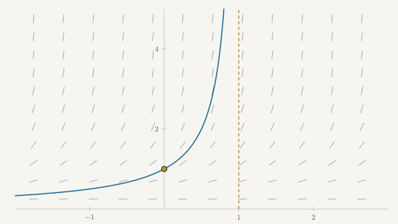
Figure 3.1 A formula reveals a lifespan. The solution of $𝑦' = 𝑦 2$ , $𝑦 (0) = 𝑦 0$ is $𝑦 = 𝑦 0 / (1 - 𝑦 0 𝑡)$ . For $𝑦 0 > 0$ , its maximal interval through $𝑡 = 0$ is $(- \infty, 1 / 𝑦 0)$ ; the dashed line marks the finite right endpoint. The slope field is smooth at every point of the plane; the finite lifespan does not come from a singularity in the slope rule. Drag the starting point: bigger starts die sooner. Beyond the asymptote the formula still has values, but the solution through $(0, 𝑦 0)$ does not.

For linear equations, our construction worked throughout the coefficient interval. For separable nonlinear equations, we first worked locally, then followed the inverse as far as it would go. Even when the equation is defined for every real time and every real value of $𝑦$ , as in $𝑦' = 𝑦 2$ , the solution may exist on a smaller time interval.

The extra hypothesis also prepares our next step. For a separable equation the local rule is $𝐹 (𝑡, 𝑦) = 𝑔 (𝑡) ℎ (𝑦)$ . Holding $𝑡$ fixed and differentiating with respect to $𝑦$ gives

𝜕 𝐹 𝜕 𝑦 (𝑡, 𝑦) = 𝑔 (𝑡) ℎ' (𝑦) .

Our stronger assumptions make both $𝐹$ and this derivative continuous. The next theorem uses these same conditions to guarantee existence and uniqueness even when separation and the product rule give us no formula.

3.3General Existence and Uniqueness

Our proofs so far used the special form of the equation to construct a solution. For a general equation $𝑦' = 𝐹 (𝑡, 𝑦)$ , we may have neither a product rule to undo nor variables we can separate. But the conditions we just encountered still give us an existence-and-uniqueness theorem.

We will write $𝐹 𝑦$ for the partial derivative $𝜕 𝐹 / 𝜕 𝑦$ , computed by holding $𝑡$ fixed and differentiating with respect to $𝑦$ . For a linear equation, $𝐹 (𝑡, 𝑦) = 𝑓 (𝑡) 𝑦 + 𝑔 (𝑡)$ , this is simply $𝐹 𝑦 (𝑡, 𝑦) = 𝑓 (𝑡)$ . For a separable equation, we just found $𝐹 𝑦 (𝑡, 𝑦) = 𝑔 (𝑡) ℎ' (𝑦)$ . In both cases, our assumptions made $𝐹$ and $𝐹 𝑦$ continuous. The following theorem applies whenever these two continuity conditions hold near the initial point, regardless of whether the equation has either special form.

Theorem 3.4 (Local existence and uniqueness). Suppose that $𝐹 (𝑡, 𝑦)$ and its partial derivative $𝜕 𝐹 𝜕 𝑦 (𝑡, 𝑦)$ are continuous in a neighborhood of $(𝑡 0, 𝑦 0)$ . Then the initial value problem

{𝑦' = 𝐹 (𝑡, 𝑦), 𝑦 (𝑡 0) = 𝑦 0

has exactly one solution on some open interval containing $𝑡 0$ .

The hypotheses are also a particularly understandable sufficient test, not the most general version of the theorem. Continuity of $𝐹$ keeps the slope rule from jumping abruptly and is enough to guarantee a local solution; continuity of $𝜕 𝐹 / 𝜕 𝑦$ controls how quickly the rule can change as the state $𝑦$ changes and guarantees uniqueness.

We will leave the proof of general existence out. But we can sketch why uniqueness holds using the linear theory we have already developed.

Proof sketch of uniqueness. The uniqueness argument has the same shape as the linear case. Suppose $𝑢$ and $𝑣$ are two solutions with the same initial value, and consider their difference $𝑤 = 𝑢 - 𝑣$ . Then

𝑤' = 𝐹 (𝑡, 𝑢) - 𝐹 (𝑡, 𝑣) .

Wherever $𝑢 \neq 𝑣$ , write this as

𝑤' = 𝑎 (𝑡) 𝑤, 𝑎 (𝑡) = 𝐹 (𝑡, 𝑢 (𝑡)) - 𝐹 (𝑡, 𝑣 (𝑡)) 𝑢 (𝑡) - 𝑣 (𝑡) .

This quotient measures how much the prescribed rate changes when we change the value of the solution. When the two values coincide, we define $𝑎 (𝑡) = 𝐹 𝑦 (𝑡, 𝑢 (𝑡))$ . The mean value theorem and continuity of $𝐹 𝑦$ ensure that this fills in the quotient continuously near the initial time.

So the difference satisfies a first-order linear equation! Since $𝑤 (𝑡 0) = 0$ , our linear uniqueness result forces $𝑤 = 0$ : the two solutions agree nearby. Wherever the theorem's hypotheses continue to hold, repeating the argument extends their agreement throughout their common interval. If the interval of agreement had an endpoint inside the solutions’ common domain, continuity would make them agree there too, and local uniqueness would extend their agreement past it.

3.4Understanding the Guarantees

The phrase “some interval” is important: this is a local theorem. It promises that a unique history begins at our chosen point, but not that the history continues forever. We have already seen this with $𝑦' = 𝑦 2$ : the rule is smooth everywhere, but the solution through $𝑦 (0) = 1$ blows up at $𝑡 = 1$ .

The hypotheses also deserve a careful reading. They are sufficient: when they hold, we get the promised conclusion. If one fails, the theorem is silent. We have to investigate the equation itself to find out whether existence or uniqueness actually fails.

Example 3.5 (A rate with a sudden switch). Consider the initial value problem

𝑦' = {0, 𝑡 < 0, 1, 𝑡 \geq 0, 𝑦 (0) = 0 .

The prescribed rate jumps at $𝑡 = 0$ , so $𝐹$ is not continuous there. Can any differentiable function obey this rule on an open interval containing zero?

Before zero, its derivative would have to be zero, so the function would be constant. After zero, its derivative would have to be one, so it would have the form $𝑡 + 𝐶$ . Continuity at zero and the initial condition force both constants to be zero. The only possible candidate is

𝑦 (𝑡) = {0, 𝑡 < 0, 𝑡, 𝑡 \geq 0 .

But this function has a corner at zero: its left derivative is zero and its right derivative is one. It is not differentiable there! Thus no solution exists on an open interval containing the initial time. A solution must satisfy the differential equation at every time in its interval, including the time when the rate switches.

What if $𝐹$ is continuous, but the derivative hypothesis fails? A local solution exists, but it need not be unique.

Example 3.6 (One point, two solutions). Consider the initial value problem

{𝑦' = 3 𝑦 2 / 3, 𝑦 (0) = 0 .

The rule $𝐹 (𝑦) = 3 𝑦 2 / 3$ is continuous at $𝑦 = 0$ , but its derivative $𝐹' (𝑦) = 2 𝑦 - 1 / 3$ is not. And indeed, both

𝑦 (𝑡) = 0 a n d 𝑦 (𝑡) = 𝑡 3

pass through the origin and satisfy the differential equation. The same initial point therefore leads to more than one possible history.

3.5Qualitative Solutions

We began this chapter wanting to say “take the solution” and investigate it, even without knowing its formula. We now have conditions which let us do that. What can we learn?

In Chapter 1, we noticed that the differential equation prescribes just one slope at each point. Two solution curves therefore cannot meet with different tangents. But that leaves a possibility: could they meet with the same tangent and then separate? They might even cross while sharing a tangent at the crossing.

Uniqueness rules out all of these possibilities. Two solutions which differ anywhere on their common interval cannot even touch.

Why? Suppose two solutions meet at time $𝑡 *$ , with

𝑢 (𝑡 *) = 𝑣 (𝑡 *) = 𝑎 .

We can treat the meeting point as an initial condition. Both functions solve

𝑦' = 𝐹 (𝑡, 𝑦), 𝑦 (𝑡 *) = 𝑎 .

Uniqueness forces them to agree near $𝑡 *$ , and the continuation argument from the preceding section extends that agreement throughout their common interval. This works in both time directions. The word “initial” does not require us to look only forward!

Corollary 3.7 (Solutions do not touch). Suppose $𝐹$ and $𝐹 𝑦$ are continuous near every point of two solution curves of $𝑦' = 𝐹 (𝑡, 𝑦)$ . If the solutions agree at one time, they agree throughout the interval where both are defined.

This gives us a way to compare solutions without finding either one. Suppose

𝑢 (𝑡 0) < 𝑣 (𝑡 0) .

Could their order ever reverse? The difference $𝑣 - 𝑢$ is continuous, so to change from positive to negative it would have to pass through zero. But then the two solutions would meet, forcing them to agree at $𝑡 0$ as well. That contradicts how they started. In fact, the same argument rules out even a moment of equality.

Thus

𝑢 (𝑡 0) < 𝑣 (𝑡 0) ⟹ 𝑢 (𝑡) < 𝑣 (𝑡)

throughout their common interval. We call this preservation of order.

The solutions might both rise, both fall, or change direction. They might move closer together or farther apart. Whatever they do, the one which starts above stays above while both exist. The equation may depend explicitly on time; nothing in the argument required the special form $𝑦' = 𝑓 (𝑦)$ .

Now a single solution we can recognize becomes useful information about all the others. Its graph acts as a barrier: solutions beginning above it stay above it, and solutions beginning below it stay below it. We do not need formulas for those other solutions to know a region they can never enter.

Some of the easiest solutions to recognize are the ones which do not move. We already looked for these in Chapter 2, before dividing by a factor that might be zero. Now they can help us understand other solutions too.

For the constant function $𝑦 (𝑡) = 𝑎$ , the derivative is zero. Thus it solves $𝑦' = 𝐹 (𝑡, 𝑦)$ precisely when

𝐹 (𝑡, 𝑎) = 0

at every time in the interval we are considering. Checking this at just one time is not enough: the equation must keep prescribing zero slope along the entire horizontal line.

Definition 3.8 (Equilibrium solutions). A constant solution $𝑦 (𝑡) = 𝑎$ of a differential equation is called an equilibrium solution, and its value $𝑎$ is called an equilibrium.

An equilibrium gives us a solution curve without any integration. But uniqueness makes that horizontal line much more useful: it becomes a barrier for every other solution.

Corollary 3.9 (Equilibria are barriers). Under the uniqueness hypotheses above, a solution which begins above an equilibrium remains strictly above it throughout their common interval of existence. A solution which begins below remains strictly below.

The proof is already contained in preservation of order: compare the solution with the constant solution $𝑦 (𝑡) = 𝑎$ . It cannot even touch the equilibrium unless it agrees with that equilibrium throughout their common interval.

Consequently, if we find two equilibria $𝑎 < 𝑏$ , any solution starting between them stays between them while it exists. We may have no formula for that solution, but we already know a region it cannot leave!

Nothing here requires the equation to be autonomous. The rate may depend on time; what matters is that the constant functions really are solutions and that uniqueness applies.

Barriers tell us where a solution can go. What can we say about how it moves there? We already know a useful test from calculus: look at the sign of its derivative. The differential equation gives us that sign without requiring us to find the solution first!

Where $𝐹 (𝑡, 𝑦) > 0$ , the slope field points upward, so a solution is increasing while it remains in that region. Where $𝐹 (𝑡, 𝑦) < 0$ , it is decreasing. If we can use solution barriers to keep a history in a region where the sign is fixed, we know its direction of motion throughout its interval of existence.

Let us return to the equation whose slope field we drew in Chapter 1:

𝑦' = 𝑡 - 𝑦 .

Below the diagonal $𝑦 = 𝑡$ , we have $𝑡 - 𝑦 > 0$ , so solutions rise. Above it, we have $𝑡 - 𝑦 < 0$ , so solutions fall. Along the diagonal itself, the assigned slope is zero.

Does that make the diagonal a solution barrier? Check it! The function $𝑦 (𝑡) = 𝑡$ has derivative $1$ , but the equation asks for $𝑡 - 𝑡 = 0$ . It is not a solution. A solution passing through this diagonal has a horizontal tangent there; it does not follow the diagonal. Uniqueness therefore gives us no reason to forbid crossing this line. Finding where $𝐹$ vanishes tells us where solutions have horizontal tangents, but those points need not themselves form a solution curve.

There is another nearby line which does solve the equation:

𝑦 (𝑡) = 𝑡 - 1 .

Its derivative is $1$ , and substituting into the right-hand side gives $𝑡 - (𝑡 - 1) = 1$ . Thus this line really is a barrier. A solution which starts below it stays below it, and one which starts above stays above, throughout their common interval. The linear theorem tells us that these solutions exist on the whole real line.

Now combine the two kinds of information. If $𝑦 (𝑡 0) < 𝑡 0 - 1$ , preservation of order gives

𝑦 (𝑡) < 𝑡 - 1

at every time. This keeps the solution below the diagonal $𝑦 = 𝑡$ , where the slopes are positive. So the solution is increasing throughout its entire history. We have learned this by checking one particularly simple solution and reading the signs of the slope field, without finding a formula for the solution we are investigating.

Let us try these ideas on some equations where the calculations are particularly simple. For an autonomous equation $𝑦' = 𝑓 (𝑦)$ , the rule does not change with time. Such equations occur frequently in scientific models, and we will meet them throughout the book. Here, their simple form makes it easy to find solution barriers and read the signs of the slopes.

For $𝑦' = 𝑓 (𝑦)$ , finding an equilibrium means solving the algebraic equation

𝑓 (𝑎) = 0 .

There is no time variable to check: once $𝑓 (𝑎) = 0$ , the constant function $𝑦 (𝑡) = 𝑎$ satisfies the differential equation at every time. Draw these equilibrium solutions as horizontal lines in the slope field. Under our uniqueness hypotheses, every other solution must stay on its own side of each line.

What happens between them? Suppose $𝑎 < 𝑏$ are two neighboring equilibria. There are no zeros of $𝑓$ between $𝑎$ and $𝑏$ , and continuity prevents $𝑓$ from changing sign without passing through zero. Thus either

𝑓 (𝑦) > 0 t h r o u g h o u t 𝑎 < 𝑦 < 𝑏,

or $𝑓 (𝑦) < 0$ throughout that interval. We can determine which by checking the sign at just one value between the roots.

Now our two general observations work together. A solution starting between $𝑎$ and $𝑏$ stays between them, and the sign tells us whether it keeps increasing or keeps decreasing. We can begin sketching its history without doing any integration!

The same sign reasoning works above the largest equilibrium or below the smallest, when those exist. There may be no second equilibrium to bound the motion, but the solution still cannot change direction while it stays in an interval where $𝑓$ has no zeros. We must keep its lifespan in mind, though: moving in one direction does not guarantee that a solution exists forever, as $𝑦' = 𝑦 2$ already showed us.

Let us try this on

𝑦' = 1 - 𝑦 2 .

The equilibria occur where $1 - 𝑦 2 = 0$ , so begin by drawing the horizontal solution lines $𝑦 = - 1$ and $𝑦 = 1$ .

Now choose an initial value between $- 1$ and $1$ . The solution cannot touch either equilibrium, so its entire history stays in this strip. And since $1 - 𝑦 2 > 0$ there, it keeps increasing. Try sketching a curve with these properties: it must follow the upward slopes while staying strictly below the horizontal line $𝑦 = 1$ .

But there is still something to justify. Must this solution actually approach $1$ ? Could it flatten out toward some smaller value instead? And do we know that its history continues for arbitrarily large times?

Our sketch suggests answers, but now it's up to us to try to pull them out of the mathematics.

The separable result settles the lifespan question. A solution increasing between $- 1$ and $1$ cannot grow without bound. Nor can its history end at a value inside the strip, where our inverse construction still works, or approach the equilibrium at $1$ in finite time. So it continues for every future time.

Since the solution increases and stays below $1$ , it must approach a limit $𝐿$ , with $- 1 < 𝑦 0 \leq 𝐿 \leq 1$ . Could $𝐿$ be smaller than $1$ ? Then $1 - 𝐿 2 > 0$ , so as the solution approaches $𝐿$ , its rate approaches a positive number. Eventually it would gain at least some fixed amount per unit time, making it impossible to settle at $𝐿$ . Thus

l i m 𝑡 \to \infty 𝑦 (𝑡) = 1 .

The same reasoning works between neighboring equilibria of any $𝑦' = 𝑓 (𝑦)$ with continuously differentiable $𝑓$ : the solution approaches the equilibrium in its direction of motion. In problem 14, you will make this argument precise for general $𝑓$ .

What happens outside this strip? Above $𝑦 = 1$ , the slopes are negative, so solutions decrease. Uniqueness keeps them above the equilibrium, and the same continuation and limit argument shows that they approach $1$ . Thus solutions on both sides pile up toward the horizontal solution $𝑦 = 1$ .

Below $𝑦 = - 1$ , the slopes are also negative, but now decreasing carries solutions away from the equilibrium. There are no further equilibria below them. Could a solution nevertheless approach some finite lower value? Our previous argument rules this out: at any such value, the rate would still be negative, keeping the solution moving downward. These solutions therefore decrease without bound.

In fact, they reach $- \infty$ in finite time: the solution ends by becoming unbounded, just as our earlier $𝑦' = 𝑦 2$ solution did by growing toward $+ \infty$ . You will prove this by separation in problem 11.

Solutions on both sides of $1$ approach it as time increases; we call this equilibrium attracting. Near $- 1$ , solutions on either side move away; we call it repelling.

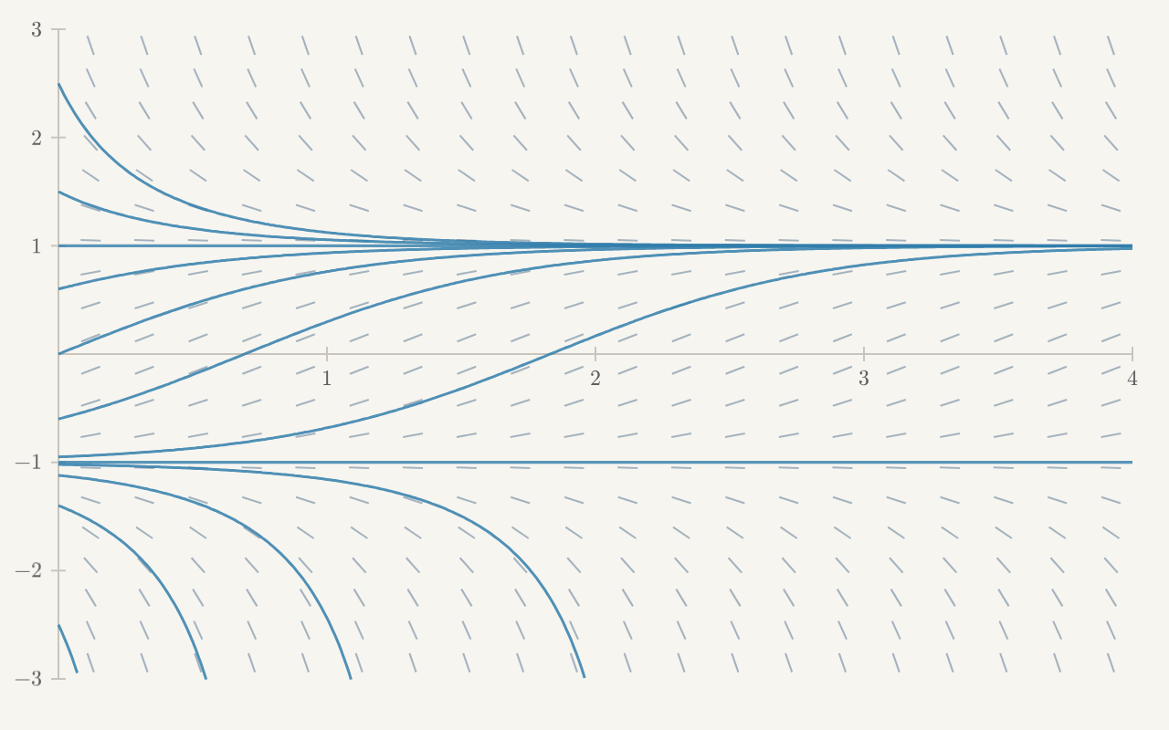
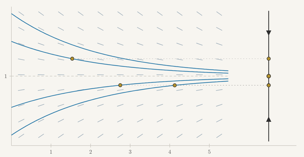
Figure 3.2 For $𝑦' = 1 - 𝑦 2$ , draw the two equilibrium histories and compare the slopes in the three regions they separate. Solutions between $- 1$ and $1$ rise toward $1$ , and those above $1$ fall toward it. Below $- 1$ , solutions fall without bound and leave the visible window before their finite lifespan ends. In the live figure, click the slope field to release a state and follow its solution.

Must an equilibrium attract from both sides or repel from both sides? Compare

𝑦' = - 𝑦 a n d 𝑦' = 𝑦 2 .

Both have their only equilibrium at zero. For the first equation, slopes are positive below zero and negative above it. Solutions on both sides move toward the equilibrium.

For $𝑦' = 𝑦 2$ , however, every slope away from zero is positive. Solutions starting below zero increase toward it, while those starting above zero increase away from it. The equilibrium attracts from one side and repels from the other. We call this behavior semistable.

The difference is visible in the algebra. In $𝑓 (𝑦) = - 𝑦$ , the factor $𝑦$ occurs once, so its sign changes across zero. In $𝑓 (𝑦) = 𝑦 2$ , the factor is squared, so the sign stays positive on both sides.

More generally, a polynomial has a simple zero at $𝑎$ when the factor $𝑦 - 𝑎$ occurs exactly once, and a double zero when it occurs exactly twice. Near a simple zero, the sign changes across the equilibrium; near a double zero, it does not. Checking those signs tells us how solutions move on each side.

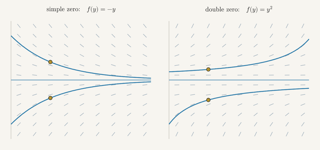
Figure 3.3 Across a simple zero, the sign of $𝑓$ changes, so the slopes tilt in opposite directions on the two sides of the equilibrium wall. Across this double zero, the sign stays positive, so the slopes tilt upward on both sides. Gold states flow toward the simple zero from both sides, but toward the double zero from below and away from it above.

We can recognize the same behavior in Newton's law of cooling, $𝑇' = - 𝑘 (𝑇 - 𝑇 r o o m)$ , with $𝑘 > 0$ . Above room temperature the rate is negative; below it the rate is positive. The equilibrium $𝑇 = 𝑇 r o o m$ is attracting, and uniqueness prevents any other solution from reaching or crossing it. Thus hot objects cool toward room temperature and cold objects warm toward it.

An equation can also have more than one attracting equilibrium. For $𝑦' = 𝑦 - 𝑦 3 = 𝑦 (1 - 𝑦) (1 + 𝑦)$ , the equilibria are $- 1$ , $0$ , and $1$ . Check the signs on either side of each: $- 1$ and $1$ are attracting, while $0$ is repelling. Every positive initial value gives a solution approaching $1$ , every negative initial value gives one approaching $- 1$ , and an initial value of zero gives the constant solution. The initial condition therefore selects between two attracting outcomes, with the equilibrium at zero separating the initial values that lead to each.

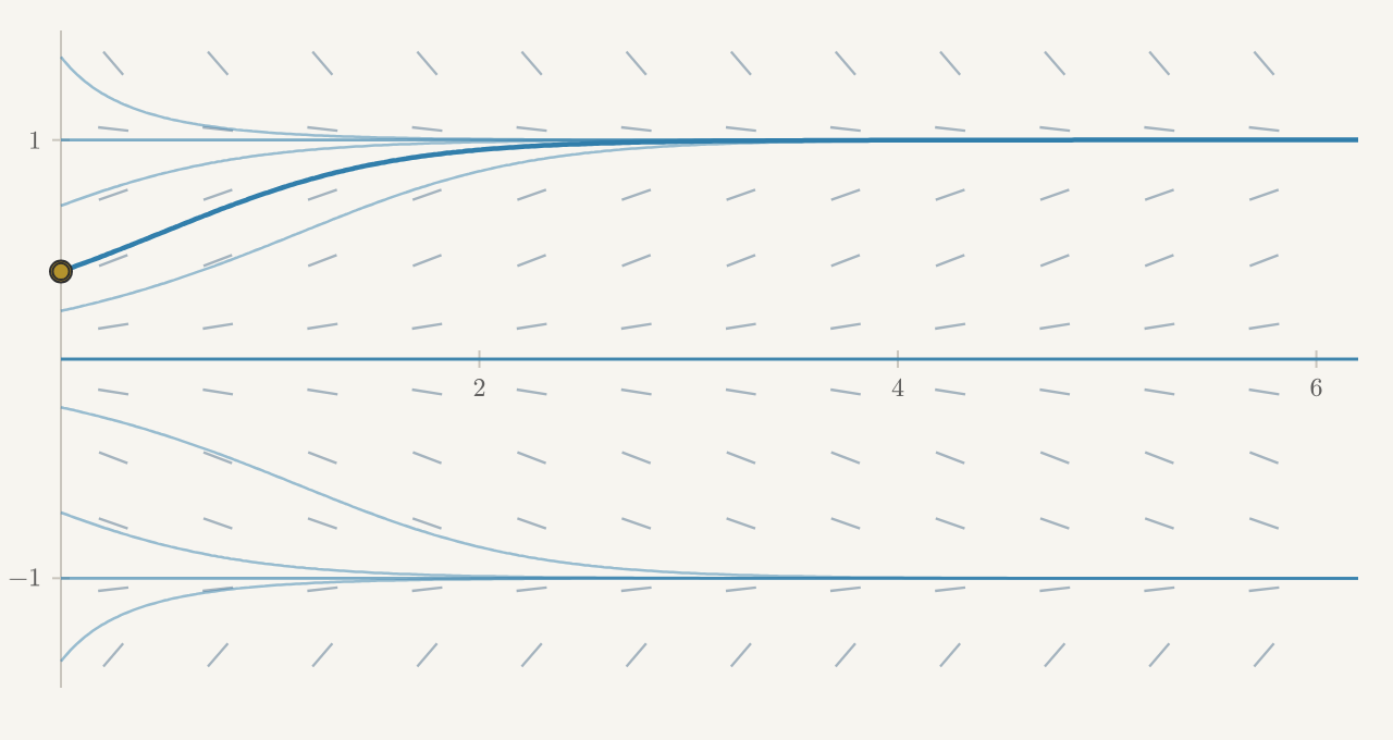
Figure 3.4 One rule, two possible destinations. For $𝑦' = 𝑦 - 𝑦 3$ , the attracting equilibria at $- 1$ and $1$ collect the histories on their side of the repelling equilibrium at $0$ . In the live figure, drag the gold initial state up and down. Its blue history changes immediately, and the moving gold point follows that history toward its equilibrium.

In each of our autonomous examples, a nonconstant solution keeps moving in one direction. This holds even when there are no equilibria to trap it between. Could a solution of $𝑦' = 𝑓 (𝑦)$ ever turn around?

To change direction, its derivative would have to pass through zero. But if $𝑦' (𝑡 *) = 0$ , then

𝑓 (𝑦 (𝑡 *)) = 0 .

The solution has reached an equilibrium! Uniqueness then forces it to agree with that constant solution throughout its interval. Thus a nonconstant solution can never have zero derivative. Since $𝑦' = 𝑓 (𝑦)$ is continuous, its sign stays fixed.

Proposition 3.10 (Nonoscillation). Suppose $𝑓$ is continuously differentiable. Every nonconstant solution of $𝑦' = 𝑓 (𝑦)$ is strictly increasing or strictly decreasing throughout its interval of existence. In particular, there are no nonconstant periodic solutions.

So if we want to model something that oscillates, like a spring, an equation of the form $𝑦' = 𝑓 (𝑦)$ won't do. For the spring we used $𝑥 ″ = - 𝑥$ : allowing a second derivative makes oscillation possible.

For the autonomous equations we have just studied, the slope field repeats the same information across every horizontal line. The slope at a given height depends only on that height. If we want, we can compress this picture onto a single copy of the $𝑦$ -axis.

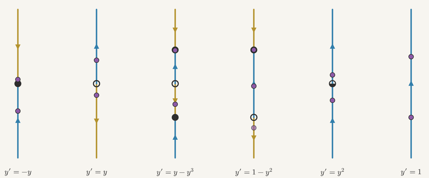
Mark the equilibria on this line. Between them, draw arrows pointing upward where $𝑓 (𝑦) > 0$ and downward where $𝑓 (𝑦) < 0$ . This picture is called a phase line. It records the equilibrium values and directions of motion that we already used to understand the solution curves.

Figure 3.5 Each moving point on a cooling solution casts a horizontal shadow onto the phase line, keeping only its current temperature. Watch the point and its shadow move together toward the room-temperature value. The arrows on the line record the direction of that motion.

Watch a point move along one of the cooling curves. Its horizontal shadow on the phase line keeps only its temperature. As the original point moves forward in time, its shadow moves toward room temperature. We can follow the same history as a curve in the slope field or as a moving point on the line.

The phase line is useful when we want to see these directions and equilibria at a glance. But the arrows alone do not tell us how long the motion takes. For $𝑦' = 1 - 𝑦 2$ , a downward arrow below $- 1$ records decreasing motion; the separation calculation tells us that the solution becomes unbounded in finite time.

Compare the phase lines below. Can you identify which equilibria attract, which repel, and which attract from only one side? Check the arrows against the signs of each equation. The final example, $𝑦' = 1$ , has no equilibria at all: every state moves upward.

Figure 3.6 Six equations, each summarized on a phase line. The arrows point upward where the rate is positive and downward where it is negative. Filled dots mark attracting equilibria, open dots mark repelling equilibria, and the half-filled dot records attraction from below and repulsion from above. The violet points move along the lines as the states change with time.

We began by asking whether we could say “take the solution” without knowing how to find it. Existence and uniqueness gave us conditions under which that makes sense. Then we put the solution to work: comparing it with other solutions, finding regions it cannot leave, and investigating where it goes as time passes. These arguments apply to whole classes of equations, even when the formulas change or disappear. In the next chapter, we will build models of our own, turning assumptions about how something works into a differential equation and investigating what it predicts.

Problems

Check Your Understanding

1What interval does the linear theorem guarantee?

Without finding solution formulas, use theorem 3.1 to answer the following.

(a)

Consider

𝑦' = (s i n 𝑡) 𝑦 + 𝑒 - 𝑡 2, 𝑦 (0) = 2 .

On what largest open interval containing the initial time does the theorem guarantee a unique solution? Identify the coefficient functions and check its hypotheses.

(b)

Answer the same question for

𝑦' = 𝑦 1 - 𝑡 + s i n 𝑡, 𝑦 (0) = 2 .

How does your answer change if the initial condition is instead $𝑦 (2) = 2$ ?

(c)

The general local existence-and-uniqueness theorem also applies near each of these initial points. What does the linear theorem tell us about the solution's interval that the local theorem alone does not?

2Reading the theorem

For each initial value problem, decide whether theorem 3.4 guarantees a unique solution near the initial point. If not, say exactly which hypothesis fails.

(a)

$𝑦' = 4 + 𝑦 3$ , with $𝑦 (0) = 1$ .

(b)

$𝑦' = \sqrt 𝑦$ , with $𝑦 (1) = 0$ ; then the same equation with $𝑦 (1) = 1$ .

(c)

$𝑦' = 𝑡 𝑦 - 2$ , with $𝑦 (0) = 2$ .

(d)

$𝑦' = | 𝑦 |$ , with $𝑦 (0) = 0$ .

3The fence

Suppose $𝐹 (𝑡, 𝑦)$ and $𝜕 𝐹 / 𝜕 𝑦$ are continuous everywhere, and suppose that $𝐹 (𝑡, 1) = 0$ for every $𝑡$ .

(a)

Show that the constant function $𝑦 (𝑡) = 1$ is a solution of $𝑦' = 𝐹 (𝑡, 𝑦)$ .

(b)

Now let $𝑦 (𝑡)$ be any solution with $𝑦 (0) = 0$ . Show that $𝑦 (𝑡) < 1$ throughout its interval of existence: the line $𝑦 = 1$ is a fence no other solution can touch.

4A solution we know tells us about solutions we don't

In Chapter 1, we checked that $𝑦 (𝑡) = 2 𝑡$ solves

𝑦' = (𝑦 - 2 𝑡) 𝑔 (𝑡, 𝑦) + 2

without needing to know the function $𝑔$ . Now suppose $𝑔$ and its partial derivative $𝑔 𝑦$ are continuous everywhere.

(a)

Verify the known solution again. Check that the right-hand side of the differential equation satisfies the hypotheses of the general existence-and-uniqueness theorem.

(b)

Let $𝑢$ and $𝑣$ be solutions with

𝑢 (0) = - 1, 𝑣 (0) = 1 .

Without finding either solution, show that

𝑢 (𝑡) < 2 𝑡 < 𝑣 (𝑡)

throughout the interval where both are defined. Explain why this holds for negative as well as positive times.

(c)

Suppose $𝑔 (𝑡, 𝑦) = - 3$ . Calculate $𝑢' (0)$ and $𝑣' (0)$ . The lower solution is initially rising and the upper solution is initially falling. Could they eventually meet? Explain how your answer fits with part (b).

5Read the phase line

Consider $𝑦' = 𝑦 (𝑦 - 2) (4 - 𝑦)$ .

(a)

Find every equilibrium and draw the phase line.

(b)

Classify each equilibrium as attracting, repelling, or semistable.

(c)

Describe the long-term fate of solutions beginning at $- 1$ , $1$ , $3$ , and $5$ without solving the equation.

(d)

Explain why none of the nonconstant solutions can oscillate.

6A periodic solution?

Suppose $𝑦$ solves $𝑦' = 𝑦$ and satisfies $𝑦 (0) = 𝑦 (1)$ .

(a)

Use the family $𝑦 = 𝐶 𝑒 𝑡$ to determine every possibility.

(b)

Give a phase-line explanation of the same conclusion which does not begin from a formula.

Explorations

7Sufficient, but not necessary

In problem 2, we saw that theorem 3.4 is silent about $𝑦' = | 𝑦 |$ , $𝑦 (0) = 0$ .

Silence is not a verdict: the theorem's hypotheses are sufficient, not necessary. Let us find out what actually happens.

(a)

Suppose a solution is positive at some time. On any interval where $𝑦 > 0$ the equation reads $𝑦' = 𝑦$ . What are the solutions of $𝑦' = 𝑦$ , and can any of them ever equal zero? If such a positive interval had a finite endpoint inside the solution's domain, what would continuity require there?

(b)

Make the corresponding argument on intervals where $𝑦 < 0$ , using $𝑦' = - 𝑦$ . Explain why a largest negative interval cannot have a finite endpoint inside the solution's domain.

(c)

Conclude that the only solution with $𝑦 (0) = 0$ is $𝑦 \equiv 0$ : uniqueness holds here even though the theorem declined to promise it. Compare with example 3.6, where the same hypothesis failed and uniqueness really was lost.

8Waiting before leaving

Consider $𝑦' = 2 \sqrt | 𝑦 |$ , $𝑦 (0) = 0$ .

(a)

Find the nonzero solutions separately in the regions $𝑦 > 0$ and $𝑦 < 0$ .

(b)

Verify that for every $𝑎 \geq 0$ , the piecewise function

𝑦 𝑎 (𝑡) = {0, 𝑡 \leq 𝑎, (𝑡 - 𝑎) 2, 𝑡 > 𝑎

solves the differential equation and initial condition.

(c)

Where does the hypothesis of theorem 3.4 fail? Explain how the family above turns that failed guarantee into visible behavior.

9Design a phase line

(a)

Construct a polynomial $𝑓 (𝑦)$ for which $𝑦' = 𝑓 (𝑦)$ has exactly three equilibria: attracting at $𝑦 = - 2$ and $𝑦 = 3$ , and repelling at $𝑦 = 0$ . Draw the phase line to check your design.

(b)

Can an autonomous equation $𝑦' = 𝑓 (𝑦)$ with continuously differentiable $𝑓$ have exactly three simple equilibria and have all three attracting? Give a sign argument.

(c)

Construct a continuously differentiable example with exactly three equilibria in which all three are attracting from at least one side. State which equilibria are semistable.

10Confident nonsense past a blowup

Euler's update does not know that the solution of $𝑦' = 𝑦 2$ , $𝑦 (0) = 1$ becomes infinite at $𝑡 = 1$ .

(a)

Use $ℎ = 0.25$ to compute $𝑦 1$ through $𝑦 6$ . What finite value does the algorithm report at $𝑡 = 1.5$ ?

(b)

Compare that table with example 3.3. Why is continuing the recursion algebraically valid but mathematically meaningless as an approximation to the original history?

(c)

State a practical warning this example gives about trusting numerical output.

11Decreasing without bound in finite time

Consider

𝑦' = 1 - 𝑦 2, 𝑦 (𝑡 0) = 𝑦 0 < - 1 .

The signs and equilibrium barriers tell us that the solution keeps decreasing below $- 1$ . We will use separation to determine how much time passes before it becomes unbounded.

(a)

Separate variables and show that, while the solution exists,

𝑡 - 𝑡 0 = \int 𝑦 (𝑡) 𝑦 0 𝑑 𝑢 1 - 𝑢 2 = \int 𝑦 0 𝑦 (𝑡) 𝑑 𝑢 𝑢 2 - 1 .

Explain why this elapsed time is positive when $𝑡 > 𝑡 0$ , even though $𝑦 (𝑡) < 𝑦 0$ .

(b)

Use partial fractions to evaluate

\int 𝑦 0 - \infty 𝑑 𝑢 𝑢 2 - 1 = 12 l o g (𝑦 0 - 1 𝑦 0 + 1) .

Check that the result is finite and positive for every $𝑦 0 < - 1$ .

(c)

Use the range of the separated integral and the maximality conclusion of theorem 3.2 to show that the right endpoint of the maximal solution interval is

𝑇 = 𝑡 0 + 12 l o g (𝑦 0 - 1 𝑦 0 + 1),

and that $𝑦 (𝑡) \to - \infty$ as $𝑡 \to 𝑇$ from below. Explain why no solution can continue this history through $𝑇$ .

Guided Proofs

12Why equilibria cannot be reached or left

Suppose $𝑔$ is continuous on an open time interval $𝐼$ , and $ℎ$ has a continuous derivative on an open interval of allowed values of $𝑦$ . Consider

𝑦' = 𝑔 (𝑡) ℎ (𝑦) .

We will prove the equilibrium claims made in the separable section using calculus. Do not invoke the general existence-and-uniqueness theorem or its consequences about solution barriers: this exercise supplies an earlier proof for separable equations.

(a)

Let $𝐽$ be a largest open interval of allowed values on which $ℎ$ never vanishes. Suppose $𝑎$ is a finite endpoint of $𝐽$ that is still inside the allowed value interval. Explain why $ℎ (𝑎) = 0$ .

Use continuity of $ℎ'$ to bound $| ℎ' |$ by some $𝑀 > 0$ near $𝑎$ . Apply the Mean Value Theorem to show that

| ℎ (𝑦) | \leq 𝑀 | 𝑦 - 𝑎 |

for $𝑦$ sufficiently close to $𝑎$ .

(b)

Fix $𝑦 * \in 𝐽$ and define

𝐻 (𝑦) = \int 𝑦 𝑦 * 𝑑 𝑢 ℎ (𝑢) .

Use the preceding bound to compare $1 / | ℎ (𝑦) |$ with $1 / (𝑀 | 𝑦 - 𝑎 |)$ . Show that integrating $1 / | ℎ (𝑦) |$ toward $𝑎$ from inside $𝐽$ gives a divergent improper integral. Why does the constant sign of $ℎ$ on $𝐽$ imply that $| 𝐻 (𝑦) | \to \infty$ as $𝑦 \to 𝑎$ from that side?

(c)

Suppose a solution takes values in $𝐽$ on a time interval containing $𝑠$ . By the chain rule and the Fundamental Theorem of Calculus,

𝐻 (𝑦 (𝑡)) - 𝐻 (𝑦 (𝑠)) = \int 𝑡 𝑠 𝑔 (𝑟) 𝑑 𝑟 .

If $𝑏$ is a finite endpoint of this time interval lying inside $𝐼$ , explain why the right side has a finite limit as $𝑡 \to 𝑏$ . Use the previous part to rule out $𝑦 (𝑡) \to 𝑎$ for any endpoint $𝑎$ of $𝐽$ inside the allowed value interval. Treat both left and right time endpoints. This also rules out approaching such an equilibrium at a finite endpoint where the solution has not yet been defined.

(d)

Let a solution be defined on an open interval $𝐾 \subseteq 𝐼$ , and suppose $ℎ (𝑦 (𝑠)) \neq 0$ at some $𝑠 \in 𝐾$ . Take $𝐽$ to be the largest interval containing $𝑦 (𝑠)$ on which $ℎ$ never vanishes. Show that $𝑦 (𝑡)$ stays in $𝐽$ for every $𝑡 \in 𝐾$ .

Hint: Take the largest time interval around $𝑠$ on which the solution stays in $𝐽$ . If it ended at a time $𝑏$ inside $𝐾$ , continuity would put $𝑦 (𝑏)$ at an endpoint of $𝐽$ inside the allowed value interval. Apply the previous part. Thus a solution starting away from equilibrium cannot reach any equilibrium at a finite time in its domain.

(e)

Now suppose $ℎ (𝑎) = 0$ and $𝑦 (𝑡 0) = 𝑎$ . Verify that $𝑦 (𝑡) = 𝑎$ is a solution on all of $𝐼$ , and prove that every solution with this initial value is constant throughout its interval.

Hint: If $𝑦 (𝑠) \neq 𝑦 (𝑡 0)$ at another time, the Mean Value Theorem gives an intermediate time $𝑟$ at which $𝑦' (𝑟) \neq 0$ . The differential equation then implies $ℎ (𝑦 (𝑟)) \neq 0$ . Apply the preceding part starting at $𝑟$ : could this same solution have the equilibrium value $𝑎$ at $𝑡 0$ ? Your argument should work whether $𝑠 < 𝑡 0$ or $𝑠 > 𝑡 0$ .

13Following the inverse as far as it works

Keep the assumptions of problem 12, and suppose $ℎ (𝑦 0) \neq 0$ . Recall the construction from the text: $𝐽$ is the largest open interval containing $𝑦 0$ among the allowed values on which $ℎ$ never vanishes, and

𝐻 (𝑦) = \int 𝑦 𝑦 0 𝑑 𝑢 ℎ (𝑢), 𝐺 (𝑡) = \int 𝑡 𝑡 0 𝑔 (𝑠) 𝑑 𝑠 .

Let $𝐼 *$ be the largest open interval containing $𝑡 0$ within $𝐼$ on which $𝐺 (𝑡) \in 𝐻 (𝐽)$ . The text proved directly that $𝑦 (𝑡) = 𝐻 - 1 (𝐺 (𝑡))$ is a solution on $𝐼 *$ . Use that construction and problem 12 to prove that this interval is maximal.

(a)

Suppose $𝑏$ is a finite endpoint of $𝐼 *$ inside $𝐼$ , and that $𝑦 (𝑡) \to ℓ \in 𝐽$ as $𝑡 \to 𝑏$ from within $𝐼 *$ . Show that $𝐺 (𝑏) = 𝐻 (ℓ)$ . Since $𝐻 (𝐽)$ is open, continuity of $𝐺$ then puts $𝐺 (𝑡)$ inside $𝐻 (𝐽)$ for times on both sides of $𝑏$ . Explain why this would extend the inverse formula beyond $𝑏$ , contradicting the choice of $𝐼 *$ .

(b)

Suppose there were a solution extending this history through a finite endpoint $𝑏$ of $𝐼 *$ inside $𝐼$ . Continuity would give a finite limit $ℓ = 𝑦 (𝑏)$ inside the allowed value interval. Explain why $ℓ$ must lie either in $𝐽$ or at an endpoint of $𝐽$ .

Rule out the first possibility using the preceding part and the second using problem 12. Notice that you only need a limit under the assumption that an extension exists; you do not need to prove that every solution has a limit at every endpoint.

(c)

Explain why an endpoint of the prescribed time interval, escape from the allowed value interval, or unbounded growth cannot permit a continuation that keeps both time and the solution values in their prescribed intervals. Treat both time directions and conclude that $𝐼 *$ is the maximal solution interval.

Finally, use the separation identity and the fact that solutions with $ℎ (𝑦 0) \neq 0$ remain in $𝐽$ to show that any solution with the same initial data agrees with $𝐻 - 1 (𝐺 (𝑡))$ and is a restriction of this maximal solution. Together with equilibrium uniqueness from the previous exercise, this completes the claims of theorem 3.2.

14Between neighboring equilibria

Suppose $𝑓$ is continuously differentiable on an open interval containing $[𝑎, 𝑏]$ , where $𝑎 < 𝑏$ , $𝑓 (𝑎) = 𝑓 (𝑏) = 0$ , and $𝑓$ has no zeros between $𝑎$ and $𝑏$ . Let $𝑦 (𝑡)$ be the maximal solution of

𝑦' = 𝑓 (𝑦), 𝑦 (𝑡 0) = 𝑦 0, 𝑎 < 𝑦 0 < 𝑏 .

We will prove that the solution exists for every future time and approaches one of the two equilibria. You may use the separable result theorem 3.2, including its conclusions about maximality and the impossibility of reaching an equilibrium in finite time.

(a)

Use preservation of order to show that $𝑎 < 𝑦 (𝑡) < 𝑏$ throughout the solution's interval of existence. Why does continuity of $𝑓$ then imply that the solution is either strictly increasing throughout this interval or strictly decreasing throughout it?

(b)

Suppose the maximal interval has a finite right endpoint $𝐵$ . Explain why monotonicity and boundedness give a limit $𝐿 \in [𝑎, 𝑏]$ as $𝑡 \to 𝐵$ from below. If $𝑎 < 𝐿 < 𝑏$ , use the inverse construction from the separable section to show that the solution extends through $𝐵$ . If $𝐿 = 𝑎$ or $𝐿 = 𝑏$ , use the equilibrium nonarrival conclusion. Deduce that the solution exists for all $𝑡 \geq 𝑡 0$ .

(c)

Show that $𝑦 (𝑡)$ has a limit $𝐿 \in [𝑎, 𝑏]$ as $𝑡 \to \infty$ . Suppose $𝑓 (𝐿) \neq 0$ . Use continuity to find a constant $𝑐 > 0$ and a time $𝑇$ such that, for all $𝑡 \geq 𝑇$ , either $𝑦' (𝑡) \geq 𝑐$ or $𝑦' (𝑡) \leq - 𝑐$ . Integrate this inequality from $𝑇$ to $𝑡$ to contradict boundedness. Conclude that $𝑓 (𝐿) = 0$ .

(d)

Use the direction of motion and the initial value to show that

l i m 𝑡 \to \infty 𝑦 (𝑡) = {𝑏, i f 𝑓 > 0 o n (𝑎, 𝑏), 𝑎, i f 𝑓 < 0 o n (𝑎, 𝑏) .

Explain why the proof does not require evaluating a separated integral or finding a formula for $𝑦 (𝑡)$ .

Python: Comparing Solution Histories

15Many initial values, one phase line

Use the Euler function from Chapter 2 to compute solutions of $𝑦' = 𝑦 - 𝑦 3$ from initial values $- 2, - 1.2, - 0.5, 0, 0.5, 1.2, 2$ .

Use $ℎ = 0.01$ through $𝑡 = 8$ . Plot the histories on one set of axes and mark the three equilibrium lines. Then make a second plot showing only the final computed value against the initial value. Explain how the two plots reveal the same two basins separated by the repelling equilibrium.

Advanced Explorations

16Dependence on initial conditions

Uniqueness tells us what happens when two initial values agree exactly. What if they are only close? For linear equations, we can calculate exactly how their difference affects the solutions.

Let $𝑓$ and $𝑔$ be continuous on an open interval $𝐼$ containing $𝑡 0$ . Suppose $𝑦$ and $̃ 𝑦$ solve the same equation

𝑦' = 𝑓 (𝑡) 𝑦 + 𝑔 (𝑡),

with initial values $𝑦 (𝑡 0) = 𝑦 0$ and $̃ 𝑦 (𝑡 0) = ̃ 𝑦 0$ . The linear theorem gives both solutions throughout $𝐼$ .

(a)

Set $𝑤 = ̃ 𝑦 - 𝑦$ . Derive a differential equation and initial condition for $𝑤$ . Explain why the prescribed contribution $𝑔 (𝑡)$ disappears when we compare the two solutions.

(b)

Use an integrating factor to prove that

̃ 𝑦 (𝑡) - 𝑦 (𝑡) = (̃ 𝑦 0 - 𝑦 0) 𝑒 \int 𝑡 𝑡 0 𝑓 (𝑠) 𝑑 𝑠 .

Hint: Set $𝐴 (𝑡) = \int 𝑡 𝑡 0 𝑓 (𝑠) 𝑑 𝑠$ and differentiate $𝑒 - 𝐴 (𝑡) 𝑤 (𝑡)$ . Use the initial value to determine the resulting constant. This should also work when $𝑤 (𝑡 0) = 0$ .

Recover uniqueness and preservation of strict order from this formula. Why can the difference never change sign?

(c)

Fix $𝑇 > 0$ with $[𝑡 0, 𝑡 0 + 𝑇] \subset 𝐼$ , and suppose $| 𝑓 (𝑡) | \leq 𝑀$ on this interval, where $𝑀 \geq 0$ . Show that

| ̃ 𝑦 (𝑡) - 𝑦 (𝑡) | \leq | ̃ 𝑦 0 - 𝑦 0 | 𝑒 𝑀 𝑇 f o r e v e r y 𝑡 \in [𝑡 0, 𝑡 0 + 𝑇] .

Hint: Bound $\int 𝑡 𝑡 0 𝑓 (𝑠) 𝑑 𝑠$ using $𝑓 (𝑠) \leq | 𝑓 (𝑠) | \leq 𝑀$ and $𝑡 - 𝑡 0 \leq 𝑇$ .

Given a tolerance $𝜀 > 0$ , show that requiring

| ̃ 𝑦 0 - 𝑦 0 | < 𝜀 𝑒 - 𝑀 𝑇

keeps the solutions within $𝜀$ of each other throughout this time interval. Explain how this gives continuous dependence on the initial value: on any fixed finite interval, we can make the solutions as close as we want by choosing their initial values sufficiently close.

(d)

Apply the difference formula to $𝑦' = - 𝑦$ and to $𝑦' = 𝑦$ , with initial values prescribed at $𝑡 0 = 0$ . In each case, describe what happens to a nonzero initial difference as time increases.

For which equation does every sufficiently small initial difference stay small for all future time? For which does every nonzero initial difference eventually exceed any fixed tolerance? Explain why both equations still have the continuous-dependence property from the preceding part. Pay attention to the distinction between fixing a finite observation interval and asking for closeness for all future time.