In the first part of the book, many of our solutions arrived with constants
attached. Antidifferentiating 𝑦′=2𝑡 gave the whole family 𝑦=𝑡2+𝐶.
Guessing and checking gave 𝑦=𝐶𝑒𝑡 for 𝑦′=𝑦, and
𝑥=𝐴cos𝑡+𝐵sin𝑡 for the spring 𝑥″=−𝑥. Even the system
𝑓′=𝑔,𝑔′=−𝑓, which the very first page of the book asked you to solve
just by thinking about it, has a whole family of solutions:
𝑓(𝑡)=𝐴cos𝑡+𝐵sin𝑡,𝑔(𝑡)=−𝐴sin𝑡+𝐵cos𝑡.
Often, our next move was to use an initial condition to pick out the
constants and study that one solution. Sometimes the formulas were already
written in terms of initial data: the logistic solution in terms of the
initial population 𝑁0, and the spring's motion in terms of its initial
position and velocity. We could see the whole family, but the problem at
hand often asked us to select one member.
Let's not do that this time. Before we impose any initial condition, an
equation already has a whole collection of solutions: for the spring, one
for every choice of 𝐴 and 𝐵. What does that collection look like, taken
all at once?
This asks us to study a set whose members are entire functions rather
than numbers. One thing we would like to know is how many numbers it
takes to single out one of its members. The
formulas suggest an answer, one constant for 𝑦′=𝑦 and two for the spring,
but many equations have no formula at all, and we would like an answer that
doesn't depend on finding one. We would also like to know what kind of set
it is. If we already know a few of its members, can we build others from
them?
That last question is one we can simply try.
5.1Function Spaces and Solution Sets
Start with the spring. We already know two of its solutions, cos𝑡 and
sin𝑡. Suppose 𝑢 and 𝑣 are any two solutions of 𝑥″=−𝑥, and add
them. Differentiation respects sums, so
(𝑢+𝑣)″=𝑢″+𝑣″=−𝑢−𝑣=−(𝑢+𝑣).
The sum is another solution! The same calculation works for a multiple
𝑐𝑢, whose second derivative is 𝑐𝑢″=−𝑐𝑢. So starting from just
cos𝑡 and sin𝑡, scaling and adding produces every function
𝐴cos𝑡+𝐵sin𝑡 in the family we wrote down. We can build new spring
solutions out of old ones as freely as we like.
Now try the same thing with 𝑦′=𝑦2, whose solutions taught us in
chapter 3 that a perfectly smooth rule can still produce finite-time
blowup. If 𝑢 and 𝑣 are two solutions, then
(𝑢+𝑣)′=𝑢′+𝑣′=𝑢2+𝑣2.
But for 𝑢+𝑣 to be another solution, the equation would require
(𝑢+𝑣)′=(𝑢+𝑣)2=𝑢2+2𝑢𝑣+𝑣2.
The extra term 2𝑢𝑣 vanishes only where one of the two solutions does.
Differentiation respects addition, but squaring does not: the sum of two
solutions follows the wrong rule. Scaling fails the same way, since
(𝑐𝑢)′=𝑐𝑢2 while the equation demands (𝑐𝑢)2=𝑐2𝑢2.
Look at what we just did. We added two whole functions, multiplied a
function by a number, and asked whether the result still solved the
equation. That is the arithmetic of vectors. A list of three numbers
counts as a vector because we can add lists and multiply them by scalars,
and linear algebra applies the same idea to matrices, polynomials, and
functions. It may have been a while since you thought of a function as a
vector, but that is exactly the viewpoint we need for studying a whole
collection of solutions at once.
A solution is always a solution on an interval. On an interval 𝐼, we
need a function with enough derivatives to make every expression in the
equation meaningful, satisfying the equation at every time in 𝐼. The
interval matters. The function 𝑦(𝑡)=1/(1−𝑡) solves 𝑦′=𝑦2 on
(−∞,1), but cannot provide a solution through 𝑡=1. A formula
and the interval on which it satisfies the equation belong together.
Fix an open interval 𝐼. If 𝑓 and 𝑔 are real-valued functions on 𝐼,
their sum and a scalar multiple are defined by
(𝑓+𝑔)(𝑡)=𝑓(𝑡)+𝑔(𝑡),(𝑐𝑓)(𝑡)=𝑐𝑓(𝑡)forevery𝑡∈𝐼.
These are pointwise operations: perform the arithmetic separately at
each input to obtain a new function. The familiar algebraic rules hold
because they hold at every input. For instance, 𝑓+𝑔=𝑔+𝑓 because
𝑓(𝑡)+𝑔(𝑡)=𝑔(𝑡)+𝑓(𝑡) for every 𝑡. The zero vector is the function
which is zero everywhere, and the additive inverse of 𝑓 is the function
−𝑓. Thus real-valued functions on a fixed interval form a vector space.
For differential equations, we need functions we can differentiate. Write
𝐶𝑘(𝐼) for the space of real-valued functions on 𝐼 with continuous
derivatives through order 𝑘. In particular, 𝐶1(𝐼) consists of
continuously differentiable functions, while 𝐶2(𝐼) requires two
continuous derivatives. These are vector spaces too: adding or scaling
functions preserves the required differentiability. We use 𝐶(𝐼) for
the space of continuous functions. The linear algebra appendix reviews
these spaces alongside the familiar spaces of numerical vectors.
These spaces are enormous! Even 𝐶𝑘(𝐼) for a fixed 𝑘 contains all
polynomials. The functions 1,𝑡,𝑡2,… are linearly independent:
a finite linear combination that vanishes throughout an interval is a
zero polynomial, so all its coefficients vanish. Consequently, 𝐶𝑘(𝐼)
contains arbitrarily large linearly independent collections. It is
infinite-dimensional; no finite list of functions can form a basis
for the whole space.
We will not need to find a basis for such a space. Its role is to hold
the functions among which we are looking for solutions. For example, the
solutions of 𝑦′=𝑦 on 𝐼 form the subset
S={𝑦∈𝐶1(𝐼):𝑦′(𝑡)=𝑦(𝑡)forevery𝑡∈𝐼}.
This notation separates the two requirements. Membership in 𝐶1(𝐼)
makes differentiation available; the condition after the colon asks that
the derivative agree with the function. We call S the
solution set, and 𝐶1(𝐼) its ambient space. For a second-order
equation we can work in 𝐶2(𝐼) instead. In each case, the equation
selects a subset of a much larger space of functions.
Systems fit into the same picture. A solution of the system
𝑓′=𝑔,𝑔′=−𝑓 from the introduction is a pair of functions, and
neither is an answer on its own: the derivative of the first must equal
the second, and the derivative of the second must equal the negative of
the first. We can regard the pair as a single vector-valued function,
𝑋(𝑡)=(𝑓(𝑡)𝑔(𝑡)).
At each time, 𝑋(𝑡) is a vector in ℝ2. The whole function
𝑋 records how that vector changes with time. Its derivative is computed
component by component, so the system can be written
𝑋′(𝑡)=(𝑓′(𝑡)𝑔′(𝑡))=(𝑔(𝑡)−𝑓(𝑡)).
This is still the same pair of equations. Collecting the functions into
a vector lets us speak of one solution while keeping track of all its
components.
More generally, a first-order system for 𝑁 unknown functions, with the
equations solved for their derivatives, has the form
𝑥′1=𝐹1(𝑡,𝑥1,…,𝑥𝑁),⋮𝑥′𝑁=𝐹𝑁(𝑡,𝑥1,…,𝑥𝑁).
Each rate may depend on every current value. Collecting the unknowns into
𝑋=(𝑥1,…,𝑥𝑁) and the known rules into 𝐹=(𝐹1,…,𝐹𝑁)
gives the compact expression 𝑋′=𝐹(𝑡,𝑋). The functions 𝐹𝑖 may contain
products, squares, or other nonlinear expressions, as they did in our
population models. They may also depend explicitly on time. Vector
notation accommodates all of these possibilities.
For systems, use 𝐶𝑘(𝐼,ℝ𝑁), the space of vector-valued
functions whose components belong to 𝐶𝑘(𝐼). Addition, scaling, and
differentiation act component by component. Notice that 𝑁 counts the
components of the value 𝑋(𝑡) at one time; it is not the dimension of
this function space. Even one component can be any of infinitely many
linearly independent functions.
5.1.1Parameters for a Family of Functions
How large is the subset selected by an equation? We can begin with the
families we already know. On ℝ, every solution of 𝑦′=𝑦
has the form 𝑦𝐶(𝑡)=𝐶𝑒𝑡. The assignment
ℝ⟶𝐶1(ℝ),𝐶⟼𝑦𝐶
takes a number and returns an entire function. Changing 𝐶 moves through
the solution set. Every solution occurs, and two different values of 𝐶
give different solutions: just evaluate at 𝑡=0 to recover 𝑦𝐶(0)=𝐶.
Thus one real number gives a coordinate for each member of this family.
Geometrically, these functions form a line through zero in function space.
They are precisely the scalar multiples of the nonzero vector 𝑒𝑡.
This line looks quite different from the collection of exponential graphs
we drew earlier. Each entire graph represents just one point of the line!
Moving along the graph means varying 𝑡 within one function. Moving
along the line in function space means varying 𝐶 to choose a different
function.
The spring gives us a family with two parameters:
𝑦𝐴,𝐵(𝑡)=𝐴cos𝑡+𝐵sin𝑡.
Its parameters can be recovered from 𝑦𝐴,𝐵(0)=𝐴 and
𝑦′𝐴,𝐵(0)=𝐵, so different pairs give different functions. These
functions form the plane spanned by the vectors cos𝑡 and sin𝑡
in 𝐶2(ℝ). Their independence is easy to check: if
𝐴cos𝑡+𝐵sin𝑡 is the zero function, its value and derivative at
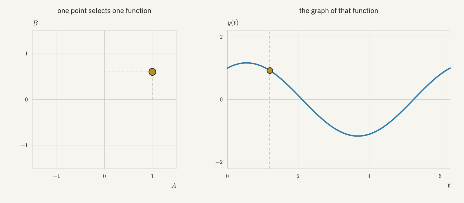
zero force 𝐴=𝐵=0. Choosing a point (𝐴,𝐵) in the parameter plane
therefore chooses one point in this plane of functions.
Figure 5.1 Choose a point (𝐴,𝐵) on the left to select the entire function
𝑦(𝑡)=𝐴cos𝑡+𝐵sin𝑡 on the right. Moving the time marker along
that graph leaves (𝐴,𝐵) fixed; moving (𝐴,𝐵) chooses a different
function. The left panel gives coordinates for functions, while the
right panel shows the values of one function over time.
This is how a differential equation can leave us with finitely many
choices even though we began in an infinite-dimensional space. We have
already verified that this whole plane consists of spring solutions.
Proving that it contains every spring solution is a further claim;
the existence-and-uniqueness theory will help us settle claims of this
kind without guessing what other functions might work.
5.1.2Linear Differential Equations
A subset of a vector space is a vector subspace if it contains zero
and is closed under linear combinations. Thus, for a solution set to be
a vector space, the zero function must solve the equation, and whenever
𝑢 and 𝑣 solve it, 𝑎𝑢+𝑏𝑣 must solve it for all real numbers 𝑎,𝑏.
The exponential line and the plane of spring solutions have this
property. Can we recognize it from the equations themselves?
Differentiation already respects the arithmetic we need:
(𝑎𝑢+𝑏𝑣)′=𝑎𝑢′+𝑏𝑣′.
In the language of linear algebra, differentiation is a linear map
from 𝐶1(𝐼) to 𝐶(𝐼). Its input is a function, and its output is
another function. More generally, a map 𝐿 between vector spaces is
linear when 𝐿(𝑎𝑢+𝑏𝑣)=𝑎𝐿(𝑢)+𝑏𝐿(𝑣). We often call a map acting on
functions an operator.
Consider the operator
𝐿:𝐶2(𝐼)⟶𝐶(𝐼),𝐿[𝑦]=𝑦″+𝑦.
It takes a function, differentiates it twice, and adds the original
function. Both operations respect linear combinations, so
Our spring equation 𝑦″=−𝑦 is exactly the equation 𝐿[𝑦]=0.
Its solutions are the functions the operator sends to zero: the
kernel of 𝐿. Recall why a kernel is a subspace. It contains zero,
and if 𝐿[𝑢]=𝐿[𝑣]=0, then
𝐿[𝑎𝑢+𝑏𝑣]=𝑎⋅0+𝑏⋅0=0. We have proved that the entire solution
set is a vector space without first finding all its members!
This reasoning works for much more than the spring. Multiplication by a
fixed function of time is also linear: for any known coefficient 𝑝(𝑡),
𝑝(𝑡)(𝑎𝑢(𝑡)+𝑏𝑣(𝑡))=𝑎𝑝(𝑡)𝑢(𝑡)+𝑏𝑝(𝑡)𝑣(𝑡). Consequently, an operator
of the form
𝐿[𝑦]=𝑎𝑛(𝑡)𝑦(𝑛)+⋯+𝑎1(𝑡)𝑦′+𝑎0(𝑡)𝑦
is linear. With continuous coefficients, it maps 𝐶𝑛(𝐼) to 𝐶(𝐼).
The coefficients can change with time; what matters is that they are
fixed functions, independent of the unknown 𝑦.
Definition 5.1 (Linear differential equations). A differential equation is linear if it can be written
𝐿[𝑢]=𝑔,
where 𝑔 is a known function and 𝐿 is a linear differential
operator: a linear map built from differentiating the unknown and
multiplying by known functions of 𝑡. We call 𝑔 the forcing. The
equation is homogeneous when 𝑔=0 and forced otherwise. An
equation that cannot be written in this form is nonlinear.
The most familiar case is a scalar equation of order 𝑛,
𝑎𝑛(𝑡)𝑦(𝑛)+⋯+𝑎1(𝑡)𝑦′+𝑎0(𝑡)𝑦=𝑔(𝑡),
whose operator is the one we just built. For example, 𝑦′=𝑦 is the
homogeneous linear equation 𝑦′−𝑦=0, and 𝑦′=𝑡𝑦 is homogeneous and
linear too: the coefficient 𝑡 varies, but the dependence on the unknown
is still linear. Squaring 𝑦 or 𝑦′ would destroy the linearity of the
corresponding operator.
For a system, consider
𝑥′=2𝑦,𝑦′=−3𝑥.
Its operator sends the pair 𝑋=(𝑥,𝑦) to
𝐿[𝑋]=(𝑥′−2𝑦,𝑦′+3𝑥). This is a linear map from
𝐶1(𝐼,ℝ2) to 𝐶(𝐼,ℝ2), and once again the
solution set is its kernel. To give this space some concrete members,
let 𝜔=√6. Direct differentiation verifies the family
Here 𝑥(0)=𝐴 and 𝑦(0)=𝐵. In checking the second equation, the
identity 𝜔2=6 makes the coefficients agree. Adding two of
these vector-valued solutions adds their parameters; multiplying a
solution by a scalar multiplies both parameters by that scalar.
The same kernel argument applies to all these equations, regardless of
their order or number of components.
Theorem 5.2 (Superposition). The solutions of a homogeneous linear differential equation or system on
a fixed interval form a vector space. In particular, if 𝑢 and 𝑣
are solutions, then 𝑎𝑢+𝑏𝑣 is a solution for every pair of real
numbers 𝑎,𝑏.
The proof is the kernel calculation above. The word linear describes
this arithmetic of functions, not the shapes of their graphs. Our
solutions can grow exponentially or oscillate while still belonging to
a vector space.
5.1.3Affine Solution Sets
What about a linear equation with a nonzero right-hand side? We have
been solving these since antidifferentiation. For example, 𝑦′=2𝑡
has the full solution family
𝑦(𝑡)=𝑡2+𝐶.
This is a line in function space too, but it does not pass through zero:
the zero function does not have derivative 2𝑡. Adding two solutions
gives 2𝑡2+𝐶1+𝐶2, whose derivative is 4𝑡, so the sum leaves
the solution set. Yet subtracting two solutions gives the constant
𝐶1−𝐶2. The direction of the line is the space of constant functions,
which solves the associated homogeneous equation 𝑦′=0.
Recall that an affine space inside a vector space is a translate
𝑝+𝑉={𝑝+𝑣:𝑣∈𝑉} of a vector subspace 𝑉. The point 𝑝
locates the translate, while 𝑉 describes its directions. Our family
𝑡2+𝐶 is the translate of the constant functions by the particular
function 𝑡2. The constants of integration were describing an affine
space all along.
The same relationship holds for every solvable linear equation. Suppose
𝐿[𝑢]=𝑔, and we have found one particular solution 𝑢𝑝. If 𝑢
is any other solution, linearity gives
𝐿[𝑢−𝑢𝑝]=𝐿[𝑢]−𝐿[𝑢𝑝]=𝑔−𝑔=0.
Thus 𝑢−𝑢𝑝 belongs to ker𝐿. Conversely, adding any homogeneous
solution ℎ∈ker𝐿 to 𝑢𝑝 gives
𝐿[𝑢𝑝+ℎ]=𝑔+0=𝑔. These two calculations establish the whole solution set:
Theorem 5.3 (The solution set of a linear equation). If 𝐿 is a linear differential operator and 𝑢𝑝 solves 𝐿[𝑢]=𝑔
on an interval 𝐼, then all solutions on 𝐼 form the affine space
𝑢𝑝+ker𝐿.
In words, every solution is one particular solution plus a solution of
the homogeneous equation.
When 𝑔=0, we can choose 𝑢𝑝=0 and recover the vector space
ker𝐿. When 𝑔 is not the zero function, zero is not a solution,
so the affine solution set is not a vector subspace. In either case,
this description assumes that a particular solution exists; it does not
yet prove existence for arbitrary equations or initial data.
5.1.4Nonlinear Solution Sets
For a linear equation, we now know which arithmetic preserves solutions:
linear combinations when the equation is homogeneous, and a particular
solution plus a homogeneous one when it is forced. The calculation for
𝑦′=𝑦2 showed that addition and scaling need not preserve solutions of
a nonlinear equation. The logistic equation 𝑦′=𝑦(1−𝑦) has the same
difficulty. For general nonlinear equations, we have no superposition
principle: knowing several solutions does not, by itself, give a way to
construct the solution from another initial state.
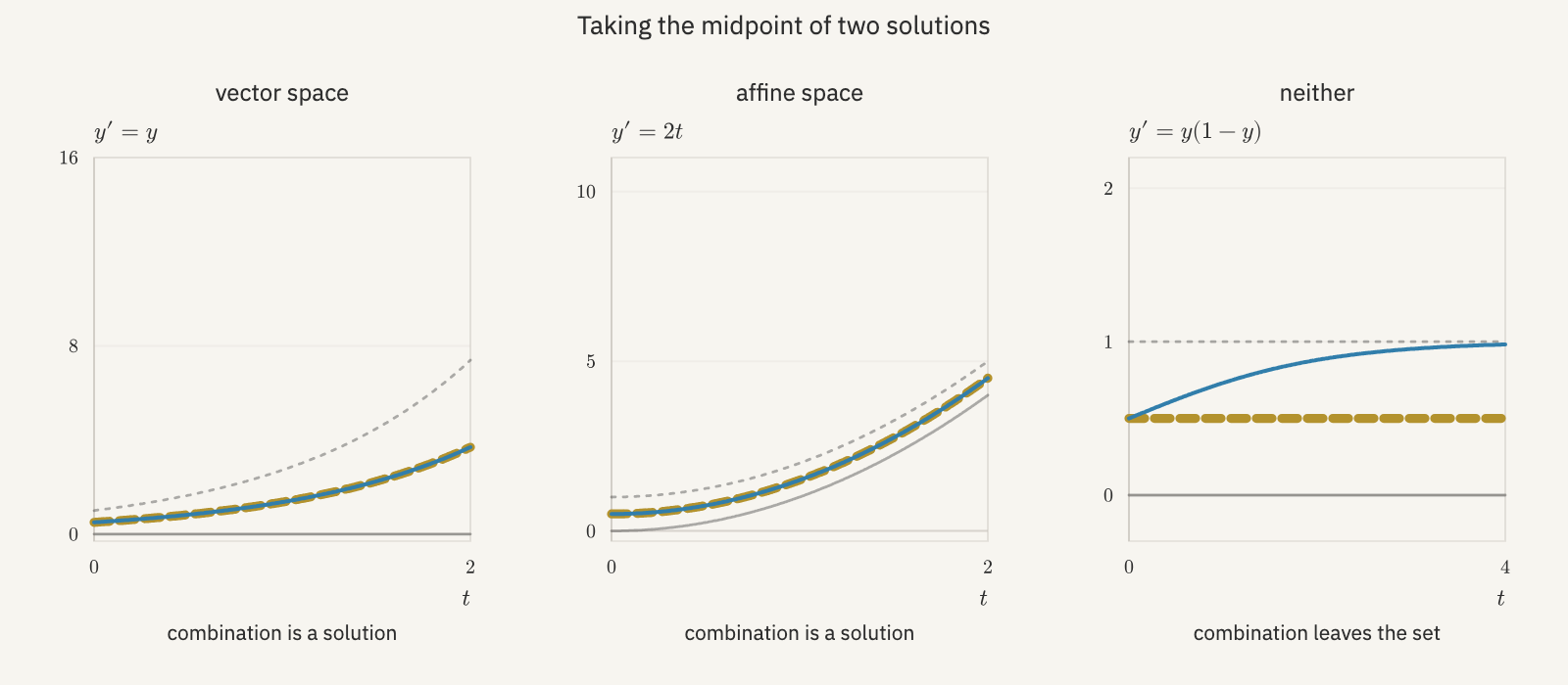
Figure 5.2 Add two solutions, or take their midpoint, and compare the result with the
solution starting at the same value. The gold dashed curve is the
combination; the blue curve is the solution. For 𝑦′=𝑦 they agree for
both operations. For the forced equation 𝑦′=2𝑡 the sum fails, but the
midpoint works, since it is still a particular solution plus a
homogeneous one. For the logistic equation, the constant solutions 𝑢=0
and 𝑣=1 have the midpoint 1/2, which is not a solution. Try other
initial values too: a combination that happens to work for one pair need
not work for every pair.
For a second-order comparison, place the spring 𝑥″=−𝑥 beside
𝑥″=1−(𝑥′)2.
Here 𝑥(𝑡)=𝑡 and 𝑥(𝑡)=−𝑡 are two solutions: each has second
derivative zero and first derivative with square one. Their sum is the
zero function, whose derivatives both vanish, so substituting it would
require 0=1. Doubling fails too: 𝑥=2𝑡 has 𝑥″=0, but
1−(𝑥′)2=−3. A nonlinear dependence on a derivative breaks the
arithmetic just as a nonlinear dependence on the function does.
Yet this equation has plenty of solutions. Here is a whole family of
them:
𝑥𝑎,𝑏(𝑡)=𝑎+log(cosh𝑡+𝑏sinh𝑡).
We do not need to discover this formula to make use of it; we can check
it. Write ℎ(𝑡)=cosh𝑡+𝑏sinh𝑡, so that ℎ″=ℎ. Wherever ℎ>0,
differentiating the proposed solution gives
𝑥′𝑎,𝑏=ℎ′ℎ,𝑥″𝑎,𝑏=ℎ″ℎ−(ℎ′ℎ)2=1−(𝑥′𝑎,𝑏)2.
The formula works. And since ℎ(0)=1 and ℎ′(0)=𝑏, its parameters
are exactly the initial data:
𝑥𝑎,𝑏(0)=𝑎,𝑥′𝑎,𝑏(0)=𝑏.
We can choose initial position and initial velocity independently, just
as we could for the spring. But they enter this family differently.
Changing 𝑎 translates the graph vertically, while changing 𝑏 changes
the function inside the logarithm. In fact, adding any constant to a
solution preserves this equation, since its derivatives do not change.
So we can obtain some new solutions from a known one. What we lack is
the freedom to combine solutions by arbitrary addition and scaling.
We still have two independent initial-data parameters, even though
they do not enter as the coefficients of two fixed solutions.
For any real 𝑎,𝑏, the formula is defined on an interval around zero,
because ℎ(0)=1. If |𝑏|≤1, it is defined for all real 𝑡:
ℎ(𝑡)=1+𝑏2𝑒𝑡+1−𝑏2𝑒−𝑡>0.
In particular, 𝑏=1 gives 𝑥=𝑎+𝑡, and 𝑏=−1 gives 𝑥=𝑎−𝑡,
recovering our earlier solutions. For |𝑏|>1, ℎ vanishes at a finite
time on one side of zero; we use the interval containing zero on which
it is positive. The parameters can affect how long a solution exists,
as well as the shape of its graph.
The spring family and the logarithmic family each use two numbers, the
initial position and velocity, to pick out one member. Their different
arithmetic does not change that count. So far, though, every count like
this has come from a formula. How many numbers pick out a solution when
there is no formula
to read them from? Chapter 3 answered this for a single first-order
equation 𝑦′=𝐹(𝑡,𝑦): under the theorem's hypotheses, one initial value
determines a unique local solution, even when we cannot find a formula.
We would like the same kind of answer for every equation we have met.
5.2A Common Formulation: First-Order Systems
We already found a connection between higher-order equations and systems
when modeling the spring. Its equation 𝑥″=−𝑥 tells us the
acceleration from the position, but position alone does not determine
the motion. Two masses can pass through the same position with different
velocities. To describe how either one moves, we need to keep track of
both quantities.
Give velocity its own name, 𝑣=𝑥′. We can now ask for the first
derivative of each quantity we are tracking. The derivative of position
is velocity, and the derivative of velocity is the acceleration supplied
by the equation:
𝑥′=𝑣,𝑣′=−𝑥.
We have replaced one second-order equation with two first-order equations.
The new variable records information the original problem already needed.
The initial conditions 𝑥(𝑡0)=𝑥0 and 𝑥′(𝑡0)=𝑣0 become the
single vector condition 𝑋(𝑡0)=(𝑥0,𝑣0) for 𝑋=(𝑥,𝑣).
Nothing about this construction required the spring equation to be
linear. Apply it to our nonlinear example 𝑥″=1−(𝑥′)2. With the
same choice 𝑣=𝑥′, we obtain
𝑥′=𝑣,𝑣′=1−𝑣2.
The second equation now involves only 𝑣, so we can solve it by
separation and then integrate 𝑥′=𝑣. The solutions 𝑥=𝑡 and
𝑥=−𝑡 correspond to the system solutions (𝑥,𝑣)=(𝑡,1) and
(𝑥,𝑣)=(−𝑡,−1). In the system, we can see why those motions work:
the velocities 1 and −1 make 𝑣′=0 and remain constant.
More generally, consider a second-order equation
𝑥″=𝐺(𝑡,𝑥,𝑥′).
The same substitution produces 𝑥′=𝑣, 𝑣′=𝐺(𝑡,𝑥,𝑣). We should
check that these descriptions really have the same solutions. If 𝑥
solves the scalar equation on an interval 𝐼, define 𝑣=𝑥′.
Then 𝑥′=𝑣 by definition, and 𝑣′=𝑥″=𝐺(𝑡,𝑥,𝑣) by the original
equation. Thus (𝑥,𝑥′) solves the system on 𝐼.
Conversely, suppose a pair (𝑥,𝑣) solves the system. Its first
equation forces 𝑣=𝑥′. Differentiating gives
𝑥″=𝑣′=𝐺(𝑡,𝑥,𝑣)=𝐺(𝑡,𝑥,𝑥′), so its first component solves the
original scalar equation. These constructions undo each other. We have
a one-to-one correspondence between the two solution sets, including
the solutions with any specified initial position and velocity. No
existence or uniqueness theorem was needed to establish this
correspondence; it follows directly from the equations.
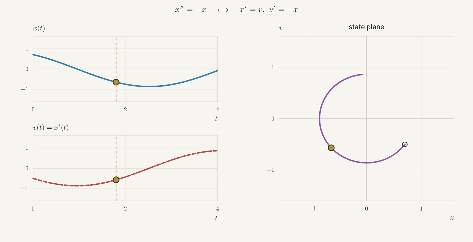
Figure 5.3 Follow one solution in its two descriptions. The graphs of 𝑥(𝑡) and
𝑣(𝑡)=𝑥′(𝑡) share a time marker; their values give the gold point
(𝑥(𝑡),𝑣(𝑡)) in the state plane. Move time to trace the same solution,
or change either initial value to choose another. Switching equations
shows the same correspondence for 𝑥″=−𝑥 and 𝑥″=1−(𝑥′)2.
Here a point in the state plane records a solution at one instant;
the entire state curve records its motion over the displayed interval.
5.2.1Recording the Derivatives
What happens for a third-order equation? Recording 𝑦 and 𝑦′ is
no longer enough to write down their rates: the derivative of 𝑦′ is
𝑦″, which the equation has not yet determined from those two values.
So record 𝑦″ too. Its derivative is 𝑦‴, and that is what the
third-order equation supplies. The construction stops when we have
recorded all derivatives below the highest one.
For an equation of order 𝑛≥2 written as
𝑦(𝑛)=𝐺(𝑡,𝑦,𝑦′,…,𝑦(𝑛−1)),
introduce the coordinates
𝑥1=𝑦,𝑥2=𝑦′,…,𝑥𝑛=𝑦(𝑛−1).
Differentiating each coordinate gives the first-order system
𝑥′1=𝑥2,𝑥′2=𝑥3,⋮𝑥′𝑛−1=𝑥𝑛,𝑥′𝑛=𝐺(𝑡,𝑥1,…,𝑥𝑛).
The first 𝑛−1 equations record the meaning of our new coordinates.
The last carries the original differential equation. Thus the state is
𝑋=(𝑦,𝑦′,…,𝑦(𝑛−1)), and prescribing its value at 𝑡0
specifies exactly the usual 𝑛 initial values for the scalar equation.
The equivalence argument works just as it did for order two. A scalar
solution produces a system solution by collecting its derivatives.
Starting with a system solution, the first equation gives 𝑥2=𝑥′1,
the next gives 𝑥3=𝑥″1, and continuing gives
𝑥𝑛=𝑥(𝑛−1)1. The last equation then says that 𝑦=𝑥1 solves
the original equation. In particular, the coordinates of a system
solution cannot be chosen as unrelated functions: the derivative
relations tie them together.
For linear equations, this conversion also preserves linearity. If
𝑎𝑛(𝑡) is nonzero, divide
𝑎𝑛𝑦(𝑛)+⋯+𝑎1𝑦′+𝑎0𝑦=𝑔 by 𝑎𝑛 to obtain the last
system equation
𝑥′𝑛=−𝑎0𝑎𝑛𝑥1−𝑎1𝑎𝑛𝑥2−⋯−𝑎𝑛−1𝑎𝑛𝑥𝑛+𝑔𝑎𝑛.
Together with the derivative chain, this is a linear system, homogeneous
when 𝑔=0. The correspondence 𝑦↦(𝑦,𝑦′,…,𝑦(𝑛−1))
itself respects addition and scaling. Our two descriptions therefore
agree about the linear or affine structure of their solution sets too.
Every first-order linear system has this shape. Collecting the
coefficients into a matrix, it reads
𝑋′=𝐴(𝑡)𝑋+𝑔(𝑡),
where 𝐴(𝑡) is an 𝑁×𝑁 matrix of known functions and 𝑔(𝑡) is a
known vector-valued function. In the language of
definition 5.1, its operator is 𝐿[𝑋]=𝑋′−𝐴(𝑡)𝑋 and its
forcing is 𝑔. The converted scalar equation is one example; the system
𝑥′=2𝑦,𝑦′=−3𝑥 from the previous section is another, with
𝐴=(02−30).
This is the form the next chapter starts from.
5.2.2Coupled Equations and the State
The same construction applies when several equations involve higher
derivatives. Suppose 𝑞=(𝑞1,…,𝑞𝑚) is a vector of unknown
functions satisfying
𝑞″=𝐺(𝑡,𝑞,𝑞′).
Record the vector 𝑣=𝑞′ along with 𝑞. We obtain 𝑞′=𝑣 and
𝑣′=𝐺(𝑡,𝑞,𝑣), a first-order system with 2𝑚 scalar coordinates.
Each component contributes its value and its first derivative to the
state. Equations with different orders work the same way: for each
unknown, record its derivatives up to one below the order of the equation
that determines its highest derivative. If those orders are
𝑛1,…,𝑛𝑚, the resulting state has
𝑁=𝑛1+⋯+𝑛𝑚 coordinates. This assumes the original system has
been solved for those highest derivatives in terms of time and the
recorded quantities.
Equations solved for their highest derivatives in this way are said to be
in normal form, and the conversion applies to them. A scalar linear
equation can be put in normal form wherever its leading coefficient
𝑎𝑛(𝑡) is nonzero; at a zero of 𝑎𝑛 we cannot divide.
Within this scope, all the equations now have the same shape:
𝑋′=𝐹(𝑡,𝑋),𝑋(𝑡0)=𝑋0,𝑋∈ℝ𝑁.
Here 𝑋 is exactly the state of definition 1.3: the current
values and derivatives we must record as initial data. The differential
equation supplies their rates of change. The starting time 𝑡0 is also
part of the initial value
problem: when 𝐹 depends explicitly on time, the same state prescribed
at different times can have different rates.
Could we reduce everything to one scalar first-order equation instead?
Even the spring shows what would be lost. At a fixed time and position,
we may choose different velocities, while a scalar equation 𝑥′=𝑓(𝑡,𝑥)
assigns just one velocity. Recording a vector allows us to retain both
initial choices. We have reduced the order by keeping more coordinates;
we have not removed the information in those coordinates.
This leaves us free to use whichever description is convenient. The
scalar equation 𝑥″=−𝑥 makes the relationship between acceleration
and position immediate, while its system makes the full state explicit.
A theorem about first-order systems can now apply to both descriptions.
The next question is whether specifying 𝑋0 actually determines a
solution: does a history begin at every initial state, and can more
than one history begin there?
5.3Existence, Uniqueness, and Initial Data
For one first-order equation, we already have a theorem that answers
this question. Continuity of the rate function and its derivative with
respect to the unknown gives local existence and uniqueness. For a
system, the corresponding hypotheses ask us to check how each component
of the rate depends on each component of the state.
Write 𝐹=(𝐹1,…,𝐹𝑁) and 𝑋=(𝑥1,…,𝑥𝑁). The partial
derivative 𝜕𝐹𝑖/𝜕𝑥𝑗 measures how the 𝑖th rate
changes as we vary the 𝑗th state coordinate, holding time and the
other coordinates fixed. There are 𝑁2 such derivatives. The theorem
has the same form in every dimension.
Theorem 5.4 (Local existence and uniqueness for systems). Suppose 𝐹(𝑡,𝑋) and all partial derivatives
𝜕𝐹𝑖/𝜕𝑥𝑗 are continuous on an open set
𝐷⊆ℝ×ℝ𝑁. For every
(𝑡0,𝑋0)∈𝐷, the initial value problem
𝑋′=𝐹(𝑡,𝑋),𝑋(𝑡0)=𝑋0
has a unique solution on a sufficiently small open interval containing
𝑡0, with (𝑡,𝑋(𝑡))∈𝐷.
We will use the system theorem without proving it. Our scalar theorem
is its 𝑁=1 case; the conversion of higher-order equations tells us
how to apply the same result far beyond that case. The hypotheses are
sufficient conditions, not a claim that every equation failing this
test must fail to have a unique solution.
For example, our nonlinear second-order equation became
𝑥′=𝑣,𝑣′=1−𝑣2.
Here 𝐹1(𝑥,𝑣)=𝑣 and 𝐹2(𝑥,𝑣)=1−𝑣2, with state derivatives
𝜕𝐹1𝜕𝑥=0,𝜕𝐹1𝜕𝑣=1,𝜕𝐹2𝜕𝑥=0,𝜕𝐹2𝜕𝑣=−2𝑣.
Everything is continuous everywhere. Thus any choice of 𝑥(𝑡0) and
𝑣(𝑡0) gives a unique local system solution. By the correspondence
we proved, any choice of 𝑥(𝑡0) and 𝑥′(𝑡0) gives a unique local
solution of the second-order equation. We have answered the question
for every initial position and velocity without solving the equation
for any of them.
The same reasoning applies to an order-𝑛 equation in normal form.
If 𝐺 and its partial derivatives with respect to
𝑦,𝑦′,…,𝑦(𝑛−1) are continuous near the prescribed data,
then the converted system satisfies the theorem's hypotheses. Each
derivative-chain equation has a coordinate as its right-hand side; only
the last equation requires us to check 𝐺. The 𝑛 prescribed
initial values therefore determine a unique local scalar solution.
Coupled higher-order equations are handled by the same check on their
combined state.
Uniqueness also settles a question we left open about the spring. We
verified that 𝑥(𝑡)=𝐴cos𝑡+𝐵sin𝑡 solves 𝑥″=−𝑥. Given any
solution on an interval containing zero, take 𝐴=𝑥(0) and 𝐵=𝑥′(0).
The displayed formula and the given solution then have the same initial
state, so uniqueness forces them to agree near zero. They agree
throughout their common interval: if agreement could stop at some time
inside that interval, their states there would agree by continuity,
and local uniqueness at that time would extend the agreement. This is
the same continuation argument we used for scalar first-order equations.
There are no missing spring solutions! The plane of functions we found
is the whole solution set on ℝ, and its restrictions give
the solutions on smaller intervals containing zero.
Existence is still a local guarantee. Even when the hypotheses hold
everywhere, a solution need not exist for all time. We already know
this from 𝑦′=𝑦2: the solution with 𝑦(0)=𝑎≠0 is
𝑦(𝑡)=𝑎/(1−𝑎𝑡) on its interval through zero, and it blows up at
𝑡=1/𝑎. Different initial values can therefore give different
intervals of existence. The theorem guarantees a history near the
initial time, not that we can follow it indefinitely. In fact, only
the zero solution of 𝑦′=𝑦2 exists on all of ℝ.
Uniqueness matters just as much. The functions 𝑦=0 and 𝑦=𝑡3
from Chapter 3 solve 𝑦′=3𝑦2/3 with the same value at zero.
For that equation, an initial value cannot distinguish the two histories.
When we use initial data to identify a solution, we are using a theorem
about the equation, not merely counting the constants in a formula.
5.3.1Initial Data as Parameters
How can finitely many numbers specify an entire function? A general
function can take values independently at many different times. A
solution of a differential equation has much less freedom: its values
must fit together according to the equation. Existence and uniqueness
tell us just how much freedom remains.
Fix an initial time 𝑡0. Under the hypotheses of our theorem, each
admissible initial state 𝜉 determines a unique local solution
𝑋𝜉, with 𝑋𝜉(𝑡0)=𝜉. Existence supplies a solution near
𝑡0. Uniqueness means that any two solutions with those data agree
throughout their common interval containing 𝑡0. Going in the other
direction is easy: given a solution defined near 𝑡0, evaluate it
there to recover the state that selected it.
The initial state therefore works as a set of coordinates for local
solutions. For an equation whose state has 𝑁 coordinates, 𝑁 numbers
recorded at a single time determine the solution near that time. This is
remarkable information to have without a solution formula: we know how
many initial values specify a solution before we have found a single one.
This answers the question we asked of our formulas. The count comes from
the equation, through its state, not from how many constants happen to
appear in a formula. We could write the solutions of 𝑦′=𝑦 as
(𝐴+𝐵)𝑒𝑡, but only the sum 𝐴+𝐵 matters. The state of 𝑦′=𝑦 has one
coordinate, and one number is what it takes.
The local qualification matters. Different initial states can give
solutions on different intervals, as the blowup of 𝑦′=𝑦2 showed.
Restricting a solution to a smaller interval containing 𝑡0 also
preserves its initial data. The data determine how the solution behaves
where it is defined; they do not prescribe which interval we write it on.
For a higher-order scalar equation, remember what these coordinates
mean. We first regard its solution as the vector-valued solution
𝑋=(𝑦,𝑦′,…,𝑦(𝑛−1)). Evaluation then records
(𝑦(𝑡0),𝑦′(𝑡0),…,𝑦(𝑛−1)(𝑡0)).
So the order-𝑛 scalar equation has a locally 𝑛-parameter solution
family under the hypotheses above. The system formulation explains why
derivative values count as parameters in exactly the same way as the
component values of a first-order system.
Return now to the nonlinear family we checked earlier:
𝑥𝑎,𝑏(𝑡)=𝑎+log(cosh𝑡+𝑏sinh𝑡),𝑥″=1−(𝑥′)2.
We verified that each function solves the equation wherever the
logarithm's argument is positive. Have we found all the solutions near
zero, or could there be others that our formula missed? Take any
solution 𝑥 on an interval containing zero and record
𝑎=𝑥(0), 𝑏=𝑥′(0). The function 𝑥𝑎,𝑏 exists near zero and
has exactly those initial data. Uniqueness forces 𝑥=𝑥𝑎,𝑏 near
zero, and the continuation argument extends their agreement throughout
their common interval. There are no missing local solutions. We did
not need a systematic method for solving the equation to establish
that our verified family was complete!
We began this chapter by asking two questions about the collection of all
solutions of an equation. What kind of set is it? Homogeneous linear
equations give vector spaces, and fixed forcing gives translates of those
spaces whenever a particular solution exists. Nonlinear equations
generally have neither structure, so the same reconstruction by linear
algebra is not guaranteed. How many initial values specify a local
solution? As many as there are coordinates in the state, for every
equation our theorem covers.
The spring and 𝑥″=1−(𝑥′)2 show that these answers are separate facts.
Both need two numbers. For the spring, those numbers select the
combination 𝑥(0)cos𝑡+𝑥′(0)sin𝑡; for the other equation, they enter
the logarithmic formula in a different way. Knowing how many numbers
we need does not tell us what arithmetic the solutions allow.
For homogeneous linear equations, these two kinds of information fit
together remarkably well. Evaluating at 𝑡0 respects addition and
scaling, and those operations keep us inside the solution set. In the
next chapter we put the two together: the initial state becomes a set
of linear coordinates for whole solutions, which will tell us the
dimension of the solution space, give us bases of solutions, and
describe evolution in time by a matrix.
Problems
The objects in this chapter live in several different spaces. A state is
a list of numbers, a solution is a function, and a solution set is a
collection of functions. Keep track of which object you are working with;
many of the calculations below become more useful once we know what they
say about the whole collection.
Check Your Understanding
1A point, a graph, and a function
Consider the family 𝑥𝐴,𝐵(𝑡)=𝐴cos𝑡+𝐵sin𝑡 of solutions to
𝑥″=−𝑥, and the corresponding system state 𝑋=(𝑥,𝑥′).
(a)
Choose (𝐴,𝐵)=(1,0). Write the resulting scalar function 𝑥(𝑡) and
vector-valued function 𝑋(𝑡). Which of these objects is a point in
𝐶2(ℝ)? Which is a point in 𝐶1(ℝ,ℝ2)?
(b)
At 𝑡=𝜋/2, record three points: the parameter point (𝐴,𝐵), the
graph point (𝑡,𝑥(𝑡)), and the state point (𝑥(𝑡),𝑥′(𝑡)). Explain
what information each point records.
(c)
Hold (𝐴,𝐵) fixed and vary 𝑡. Which of those points moves? Then
hold 𝑡=𝜋/2 fixed and vary 𝐴. Are you moving along one solution
or selecting different solutions? Use figure 5.1 to check
your interpretation.
2How many independent parameters?
(a)
The formulas 𝑦𝐶(𝑡)=𝐶𝑒𝑡 and 𝑧𝐴,𝐵(𝑡)=(𝐴+𝐵)𝑒𝑡 describe
families in 𝐶1(ℝ). Do they describe the same set of
functions? Give two different pairs (𝐴,𝐵) that describe the same
function, and explain how many independent parameters the set has.
(b)
Show that if 𝐴cos𝑡+𝐵sin𝑡=𝐶cos𝑡+𝐷sin𝑡 for every 𝑡,
then 𝐴=𝐶 and 𝐵=𝐷. Which two measurements of a function recover
its parameters?
(c)
For |𝑎|<1, consider 𝑦𝑎(𝑡)=𝑎/(1−𝑎𝑡) on (−1,1). Recover
𝑎 from the function and show that different parameters give different
functions. Does having one independent parameter imply that this family
is a vector subspace? Test a specific pair or a scalar multiple.
(d)
In 𝑦(𝑡)=𝐶𝑒𝑟𝑡, explain the different roles of 𝐶 and 𝑟 when
we are describing solutions of the fixed equation 𝑦′=2𝑦.
3Recognizing linear structure
For each equation in parts (a)–(d), decide whether it is linear as
written. If it is, identify its linear differential operator and forcing,
and decide whether it is homogeneous. State what this tells you about
its nonempty solution set on a common interval. If it is nonlinear,
identify the term that prevents the linear-operator argument from applying.
(a)
𝑦″+𝑡2𝑦′−sin(𝑡)𝑦=0.
(b)
𝑦′+3𝑦=𝑒−𝑡.
(c)
𝑦″+𝑦2=0.
(d)
𝑥′=𝑡𝑥−2𝑦, 𝑦′=𝑥+(1+𝑡2)𝑦.
(e)
For 𝑦′=𝑦(1−𝑦), use the constant solutions zero and one to prove
that the solution set on ℝ is not affine. Why would merely
finding the zero solution be insufficient to decide its structure?
4Arithmetic in an affine solution set
Let 𝐿 be a linear differential operator, and suppose 𝑢 and 𝑣
solve 𝐿[𝑦]=𝑔 on the same interval. Assume 𝑔 is not the zero
function.
(a)
Calculate 𝐿[𝑢−𝑣] and 𝐿[𝑢+𝑣]. Which equation does each function
solve? Explain why the failure of addition here does not mean 𝐿 is
nonlinear.
(b)
For real constants 𝑎,𝑏, show that 𝑎𝑢+𝑏𝑣 solves 𝐿[𝑦]=𝑔 if
and only if 𝑎+𝑏=1. What changes when 𝑔=0?
(c)
Suppose 𝑢𝑝 is one solution of 𝐿[𝑦]=𝑔. Prove that every
solution is 𝑢𝑝+ℎ for some ℎ∈ker𝐿, and that every such
function is a solution.
(d)
Apply the description to 𝑦′=2𝑡. Identify a particular solution and
the homogeneous solution space. Choose two distinct solutions and
calculate their difference and their midpoint.
5Write the state, then recover the equation
In each conversion, name every state coordinate and specify how the
initial data translate. Do not solve the equations.
(a)
Convert 𝑥″=1−(𝑥′)2, with 𝑥(0)=𝑎 and 𝑥′(0)=𝑏, to a
first-order system. Starting instead from a solution of your system,
show directly that its first component solves the scalar equation.
(b)
Convert
𝑦‴+𝑎2(𝑡)𝑦″+𝑎1(𝑡)𝑦′+𝑎0(𝑡)𝑦=0
to a first-order system. Write its initial state in terms of
𝑦(0), 𝑦′(0), and 𝑦″(0).
(c)
Convert the coupled equations
𝑥″=−𝑥+𝑦,𝑦″=𝑥−𝑦
to a first-order system. How many scalar coordinates does its state
have? List the initial data, and explain how a system solution recovers
both original equations.
(d)
For the equation 𝑎2(𝑡)𝑦″+𝑎1(𝑡)𝑦′+𝑎0(𝑡)𝑦=𝑔(𝑡), what condition
on 𝑎2 lets you carry out the usual conversion throughout an
interval? Explain which step can fail at a zero of 𝑎2.
6What does the theorem tell us?
Apply theorem 5.4. Check the right-hand side and its
state partial derivatives; do not infer uniqueness merely from how many
initial values have been supplied.
(a)
For 𝑥′=2𝑦, 𝑦′=−3𝑥, check the four state partial derivatives.
Does the theorem apply at every initial state? State precisely its
conclusion about the interval of existence.
(b)
Repeat for 𝑥′=𝑣, 𝑣′=1−𝑣2. Translate the conclusion into a
statement about initial value problems for the scalar second-order
equation.
(c)
Regard 𝑦′=3𝑦2/3 as a one-component system, where
𝑦2/3=(3√𝑦)2. Compare the initial values 𝑦(0)=1
and 𝑦(0)=0. Where does the theorem apply? At zero, verify two
distinct solutions with the same initial value. Distinguish the failed
hypothesis from the separate calculation establishing nonuniqueness.
7Have we found every solution?
For the system 𝑥′=2𝑦, 𝑦′=−3𝑥, let 𝜔=√6 and
consider the proposed family
Verify both differential equations. Recover 𝐴 and 𝐵 by evaluating
the solution at zero.
(b)
Let (𝑢,𝑣) be any solution on an interval containing zero. Choose
𝐴,𝐵 from its initial state and use uniqueness to prove that it
agrees with the displayed solution near zero. Explain why agreement
extends throughout the common interval.
(c)
Write the solution with initial state (𝑥(0),𝑦(0))=(2,−1). Which
part of your argument shows that the formula works, and which shows
that there are no other solutions with those data?
8The interval changes the solution set
For 𝑦′=𝑦2, the solution starting at 𝑦(0)=𝑎 is
𝑦𝑎(𝑡)=𝑎1−𝑎𝑡
on its interval of existence containing zero.
(a)
For which real values of 𝑎 is this solution defined throughout
(−1,1)? Include the endpoint values of your parameter range if they
work. How does the answer change if the solution must exist on an open
interval containing the closed interval [−1,1]?
(b)
Answer the first question for (−2,2), then for ℝ.
Explain why a one-parameter local family need not remain a one-parameter
family when we require solutions for all time.
Explorations
9Can solution graphs cross?
Consider the two spring solutions 𝑢(𝑡)=sin𝑡 and 𝑣(𝑡)=−sin𝑡.
(a)
Verify that both solve 𝑥″=−𝑥. Find their graph intersections and
compare their derivatives at those times.
(b)
Write the corresponding state histories 𝑈=(𝑢,𝑢′) and 𝑉=(𝑣,𝑣′).
At a time when the scalar graphs cross, do the system solutions have
the same state? Explain why uniqueness permits the graph crossings.
(c)
Could two distinct spring solutions have both the same value and the
same derivative at the same time? Give an argument using the system
theorem rather than the explicit solution formula.
(d)
Show that 𝑈 and 𝑉 trace the same unit circle in the state plane,
but never occupy the same point at the same time. Explain the
distinction between a geometric curve and a function of time. Why
does tracing the same curve not contradict uniqueness?
10How long does the nonlinear family exist?
Return to
𝑥𝑎,𝑏(𝑡)=𝑎+logℎ𝑏(𝑡),ℎ𝑏(𝑡)=cosh𝑡+𝑏sinh𝑡,
which solves 𝑥″=1−(𝑥′)2 wherever ℎ𝑏>0. We want the largest
open interval containing zero on which this formula gives a solution.
(a)
Use the exponential definitions of cosh and sinh to write
ℎ𝑏(𝑡) as a linear combination of 𝑒𝑡 and 𝑒−𝑡.
Show that ℎ𝑏(𝑡)>0 for every real 𝑡 when |𝑏|≤1.
What are the solutions when 𝑏=1 and 𝑏=−1?
(b)
When 𝑏>1 or 𝑏<−1, find the time 𝑡∗ at which ℎ𝑏(𝑡∗)=0.
Determine on which side of 𝑡∗ the function is positive, and give
the requested interval of existence in each case.
(c)
What happens to 𝑥𝑎,𝑏(𝑡) as 𝑡 approaches 𝑡∗ from inside
that interval? Explain why the solution cannot extend through 𝑡∗
as a real-valued solution, even though the system's right-hand side and
all its state partial derivatives are continuous everywhere.
(d)
Which initial states (𝑎,𝑏) give solutions for every real 𝑡?
Which give solutions for every 𝑡≥0? Sketch both sets in the
initial-data plane. Explain why changing 𝑎 does not change the
interval of existence.