Chapter 6

Linear Evolution

In chapter 5, initial data became coordinates for whole solutions. We could specify a function by finitely many numbers because the differential equation and uniqueness determined everything else. For a nonlinear equation, those coordinates pick out solutions, but the solutions they pick out cannot be combined. For a homogeneous linear equation, the solutions form a vector space. What happens when we put these two facts together?

The coordinates become linear coordinates: adding initial states adds the corresponding solutions, and scaling an initial state scales its entire solution. This means that a basis of states can give us a basis of functions. Once we have solved from those few initial states, every other initial value problem can be answered by linear algebra.

We will develop this for systems whose coefficients may depend on time. The solutions need not have convenient formulas. The point of the structure is that we can use it even when finding individual solutions is difficult.

6.1Initial Data as Linear Coordinates

Consider an $𝑁$ -component homogeneous linear system

𝑋' = 𝐴 (𝑡) 𝑋,

where $𝐴 (𝑡)$ is an $𝑁 \times 𝑁$ matrix with continuous entries on an open interval $𝐼$ . Fix $𝑡 0 \in 𝐼$ . From the last chapter, we know that every initial state gives a unique local solution. We also know that linear combinations of solutions remain solutions wherever they are all defined.

For linear equations, we can strengthen the existence conclusion: the unique solution extends throughout the interval on which the coefficients are continuous. The same strengthening holds with a continuous forcing term. The improvement concerns how long the solution exists: the local guarantee from chapter 5 becomes a guarantee on all of $𝐼$ .

Theorem 6.1 (Global existence and uniqueness for linear systems). Suppose the entries of $𝐴 (𝑡)$ and the components of $𝑔 (𝑡)$ are continuous on an open interval $𝐼$ , and let $𝑡 0 \in 𝐼$ . For every $𝑋 0 \in ℝ 𝑁$ , the initial value problem

𝑋' = 𝐴 (𝑡) 𝑋 + 𝑔 (𝑡), 𝑋 (𝑡 0) = 𝑋 0

has exactly one solution on all of $𝐼$ .

We use this theorem without proof. The word global means throughout $𝐼$ : a solution cannot blow up at a finite time inside the interval where its coefficients and forcing remain continuous. If those functions are continuous on all of $ℝ$ , every solution exists for all real time. This is the system version of the stronger linear existence theorem from chapter 3. The constant-coefficient construction in the next chapter will give an explicit special case; the theorem here also covers coefficients that vary with time.

Return to the homogeneous equation $𝑋' = 𝐴 (𝑡) 𝑋$ , and let

S (𝐼) = {𝑋 \in 𝐶 1 (𝐼, ℝ 𝑁) : 𝑋' = 𝐴 (𝑡) 𝑋} .

This is a vector subspace of the function space $𝐶 1 (𝐼, ℝ 𝑁)$ . Evaluation at $𝑡 0$ defines a map

𝐸 𝑡 0 : S (𝐼) ⟶ ℝ 𝑁, 𝐸 𝑡 0 (𝑋) = 𝑋 (𝑡 0) .

The previous chapter used this map to recover the parameters of a solution. Now both its domain and codomain are vector spaces. Does it respect their arithmetic? For any solutions $𝑈, 𝑉$ and real numbers $𝑎, 𝑏$ ,

𝐸 𝑡 0 (𝑎 𝑈 + 𝑏 𝑉) = (𝑎 𝑈 + 𝑏 𝑉) (𝑡 0) = 𝑎 𝑈 (𝑡 0) + 𝑏 𝑉 (𝑡 0) = 𝑎 𝐸 𝑡 0 (𝑈) + 𝑏 𝐸 𝑡 0 (𝑉) .

Yes! Evaluation is linear. Existence and uniqueness give the rest.

Theorem 6.2 (Initial data as linear coordinates). Let $𝐴 (𝑡)$ have continuous entries on an open interval $𝐼$ , and fix $𝑡 0 \in 𝐼$ . Evaluation at $𝑡 0$ is a linear isomorphism from the solution space of $𝑋' = 𝐴 (𝑡) 𝑋$ onto $ℝ 𝑁$ . Consequently,

d i m S (𝐼) = 𝑁 .

Proof. We have just checked linearity. For every $𝑋 0 \in ℝ 𝑁$ , existence supplies a solution $𝑋 \in S (𝐼)$ with $𝐸 𝑡 0 (𝑋) = 𝑋 0$ , so evaluation is surjective. If two solutions have the same image, they have the same initial state; uniqueness says they are the same solution on $𝐼$ . Thus evaluation is also injective.

A bijective linear map is a linear isomorphism. Isomorphic vector spaces have the same dimension, so $d i m S (𝐼) = 𝑁$ . ∎

We have determined the dimension without finding a single solution formula. The surrounding function space is infinite-dimensional, but the equation selects a subspace with exactly as many dimensions as there are state coordinates. And we know a concrete isomorphism: to turn a solution into a vector of numbers, evaluate it at $𝑡 0$ .

Suppose $𝑈$ and $𝑉$ have initial states $𝑈 0$ and $𝑉 0$ at $𝑡 0$ . Superposition says that $𝑎 𝑈 + 𝑏 𝑉$ is a solution, and its initial state is $𝑎 𝑈 0 + 𝑏 𝑉 0$ . Uniqueness therefore identifies it as the solution from that initial state. The same coefficients combine the initial states and the entire solutions.

6.1.1Higher-Order and Forced Equations

For a homogeneous scalar equation

𝑎 𝑛 (𝑡) 𝑦 (𝑛) + 𝑎 𝑛 - 1 (𝑡) 𝑦 (𝑛 - 1) + \dots + 𝑎 1 (𝑡) 𝑦' + 𝑎 0 (𝑡) 𝑦 = 0,

suppose all coefficients are continuous on $𝐼$ and $𝑎 𝑛$ never vanishes there. The conversion from chapter 5 gives an $𝑛$ -component homogeneous linear system with continuous coefficients. The correspondence $𝑦 \mapsto (𝑦, 𝑦', \dots, 𝑦 (𝑛 - 1))$ is itself linear, so the scalar solution space is $𝑛$ -dimensional. Its initial-data isomorphism records

𝑦 ⟼ (𝑦 (𝑡 0), 𝑦' (𝑡 0), \dots, 𝑦 (𝑛 - 1) (𝑡 0)) .

For a scalar equation, evaluating only $𝑦 (𝑡 0)$ would lose information. The derivative values are the remaining state coordinates.

With a fixed continuous forcing, we obtain an affine space instead. For $𝑋' = 𝐴 (𝑡) 𝑋 + 𝑔 (𝑡)$ , the existence theorem supplies a particular solution $𝑋 𝑝$ on $𝐼$ . Chapter 5 then identifies the full solution set as

𝑋 𝑝 + S (𝐼) .

Its affine dimension is $𝑁$ , the dimension of its space of directions $S (𝐼)$ . If we choose $𝑋 𝑝 (𝑡 0) = 0$ and let $𝑈$ be the homogeneous solution with $𝑈 (𝑡 0) = 𝑋 0$ , then $𝑋 𝑝 + 𝑈$ solves the forced equation with initial state $𝑋 0$ . The same reasoning gives affine dimension $𝑛$ for the scalar order- $𝑛$ forced equation under the coefficient assumptions above. These statements concern all solutions of the equation; prescribing the full initial data selects just one of them. Methods for finding particular forced solutions will come later.

6.2Bases of Solutions and Reconstruction

An isomorphism transports a basis from one vector space to another. Choose a basis $𝑏 1, \dots, 𝑏 𝑁$ of $ℝ 𝑁$ , and let $𝑈 𝑗$ be the solution with $𝑈 𝑗 (𝑡 0) = 𝑏 𝑗$ . These functions form a basis of $S (𝐼)$ . To express an arbitrary solution in that basis, we only need to express its initial state in the basis $𝑏 1, \dots, 𝑏 𝑁$ .

Theorem 6.3 (A basis of states gives a basis of solutions). Let $𝑈 1, \dots, 𝑈 𝑁$ solve the same homogeneous linear system $𝑋' = 𝐴 (𝑡) 𝑋$ on an open interval $𝐼$ , with $𝐴$ continuous and $𝑡 0 \in 𝐼$ . They form a basis of the solution space if and only if $𝑈 1 (𝑡 0), \dots, 𝑈 𝑁 (𝑡 0)$ form a basis of $ℝ 𝑁$ .

For such a basis, the unique solution from $𝑋 (𝑡 0) = 𝑋 0$ is

𝑋 (𝑡) = 𝑐 1 𝑈 1 (𝑡) + \dots + 𝑐 𝑁 𝑈 𝑁 (𝑡),

where the coefficients are determined by

𝑋 0 = 𝑐 1 𝑈 1 (𝑡 0) + \dots + 𝑐 𝑁 𝑈 𝑁 (𝑡 0) .

Proof. Evaluation is a linear isomorphism, so it preserves linear independence and spanning in both directions. For the reconstruction formula, superposition says that $𝑐 1 𝑈 1 + \dots + 𝑐 𝑁 𝑈 𝑁$ is a solution. The equation for the coefficients makes its initial state $𝑋 0$ , so uniqueness identifies it as the solution from $𝑋 0$ . The coefficients are unique because the chosen initial states form a basis. ∎

The independence assertion is worth interpreting. We can test whether whole functions are independent by examining their states at a single time. For arbitrary functions, that would be false: many different functions pass through the same value. Here uniqueness is built into the isomorphism. A linear combination of solutions that has zero initial state must be the zero solution everywhere on $𝐼$ .

Return to the oscillator from chapter 5,

𝑥' = 2 𝑦, 𝑦' = - 3 𝑥 .

With $𝜔 = \sqrt 6$ , we already know the two solutions

𝑈 (𝑡) = ⎛ ⎜ ⎜ ⎜ ⎝ c o s (𝜔 𝑡) - 3 𝜔 s i n (𝜔 𝑡) ⎞ ⎟ ⎟ ⎟ ⎠, 𝑉 (𝑡) = ⎛ ⎜ ⎜ ⎜ ⎝ 2 𝜔 s i n (𝜔 𝑡) c o s (𝜔 𝑡) ⎞ ⎟ ⎟ ⎟ ⎠ .

Their initial states are $𝑈 (0) = (1, 0)$ and $𝑉 (0) = (0, 1)$ , so the basis theorem immediately identifies them as a basis of solutions. For initial state $(𝑎, 𝑏)$ , the entire solution is $𝑎 𝑈 + 𝑏 𝑉$ . For example, $(2, - 1) = 2 (1, 0) - (0, 1)$ gives

𝑋 (𝑡) = 2 𝑈 (𝑡) - 𝑉 (𝑡) = ⎛ ⎜ ⎜ ⎜ ⎜ ⎜ ⎝ 2 c o s (𝜔 𝑡) - 2 𝜔 s i n (𝜔 𝑡) - 6 𝜔 s i n (𝜔 𝑡) - c o s (𝜔 𝑡) ⎞ ⎟ ⎟ ⎟ ⎟ ⎟ ⎠ .

There was no new integration to perform. We used two solved functions and a calculation in $ℝ 2$ . The theorem tells us that this procedure reaches every solution, and that each one has unique coefficients. Nothing in its proof required sine and cosine formulas.

6.2.1Solve a Few Times, Solve Them All

We can use the same structure when solutions must be approximated numerically. Consider the synthetic time-dependent system

𝑥' = - 14 𝑥 + (2 + 14 s i n 𝑡) 𝑦, 𝑦' = - (2 + 14 c o s 𝑡) 𝑥 - 14 𝑦 .

Without the sine and cosine perturbations, its rate is $- 14 (𝑥, 𝑦) + (2 𝑦, - 2 𝑥)$ : an inward radial component plus a clockwise turning component. The perturbations make the turning coefficients vary differently with time. This is a mathematical example chosen to explore reconstruction with time-dependent coefficients. All coefficients are continuous on $ℝ$ , so its solution space is two-dimensional and every solution exists for all real time.

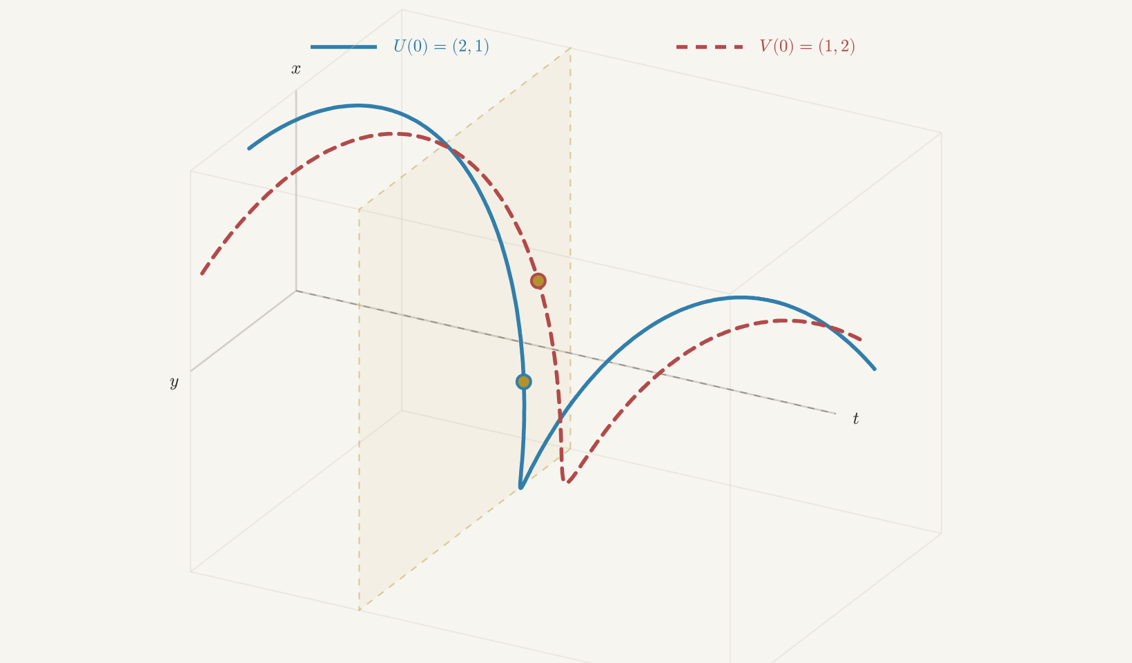
Let $𝑈, 𝑉$ now denote this system's solutions from $𝑈 (0) = (2, 1)$ and $𝑉 (0) = (1, 2)$ . These initial vectors are independent, so the solutions form a basis. We can approximate the functions and save their values on a common time grid.

Figure 6.1 The curves approximate $𝑡 \mapsto (𝑡, 𝑈 (𝑡))$ and $𝑡 \mapsto (𝑡, 𝑉 (𝑡))$ in $(𝑡, 𝑥, 𝑦)$ -space. Rotate the picture to inspect their shape, then drag the common time marker to compare their states at the same time. Keeping the time coordinate visible lets us read each curve as a function of time.

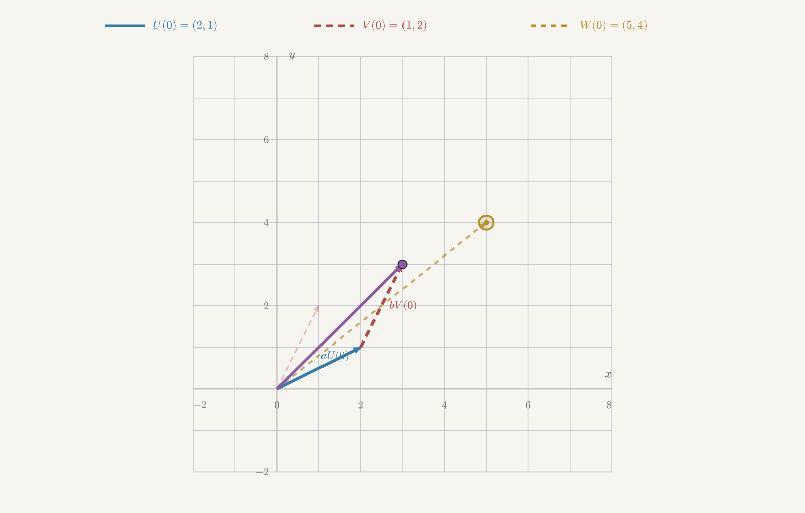
To reconstruct the solution from $(5, 4)$ , solve

𝑎 (2, 1) + 𝑏 (1, 2) = (5, 4) .

This gives $2 𝑎 + 𝑏 = 5$ , $𝑎 + 2 𝑏 = 4$ , hence $𝑎 = 2$ , $𝑏 = 1$ . The exact solution is $2 𝑈 + 𝑉$ . Combining the stored approximations with those same coefficients gives an approximation to it.

Figure 6.2 The blue and red vectors are the known initial states $𝑈 (0)$ and $𝑉 (0)$ ; the gold vector is the target $(5, 4)$ . Adjust $𝑎, 𝑏$ until $𝑎 𝑈 (0) + 𝑏 𝑉 (0)$ reaches the target. Those coefficients also combine the entire solutions.

For comparison, numerical approximations at $𝑡 = 2$ give

𝑈 (2) \approx (- 1.082775, 0.853062), 𝑉 (2) \approx (- 1.378345, 0.066657) .

The table compares reconstruction with separate numerical integrations from three initial states. Values were combined before rounding.

$𝑋 (0)$	$(𝑎, 𝑏)$	$𝑎 𝑈 (2) + 𝑏 𝑉 (2)$	direct solve at $𝑡 = 2$
$(5, 4)$	$(2, 1)$	$(- 3.543895, 1.772781)$	$(- 3.543895, 1.772781)$
$(1, - 1)$	$(1, - 1)$	$(0.295570, 0.786404)$	$(0.295570, 0.786404)$
$(0, 3)$	$(- 1, 2)$	$(- 1.673915, - 0.719747)$	$(- 1.673915, - 0.719747)$

Try this with Euler's method: compute from $(2, 1)$ and $(1, 2)$ using the same grid, then combine the stored values to approximate a third solution. Why should this agree with a direct Euler run? Write the system as $𝑋' = 𝐴 (𝑡) 𝑋$ . Its update is itself linear:

𝑋 𝑛 + 1 = (𝐼 + ℎ 𝐴 (𝑡 𝑛)) 𝑋 𝑛 .

If $𝑋 𝑛 = 𝑎 𝑈 𝑛 + 𝑏 𝑉 𝑛$ , then

𝑋 𝑛 + 1 = (𝐼 + ℎ 𝐴 (𝑡 𝑛)) (𝑎 𝑈 𝑛 + 𝑏 𝑉 𝑛) = 𝑎 𝑈 𝑛 + 1 + 𝑏 𝑉 𝑛 + 1 .

The equality holds initially, so induction gives it at every step. Apart from floating-point roundoff, combining Euler approximations on the same grid gives exactly the same discrete answer as another Euler run. Its accuracy against the true solution is a separate question, still governed by the step size and numerical error. Agreement between two ways of computing the same approximation does not eliminate that error.

6.2.2Choosing the Standard Initial States

Our numerical basis began at $(2, 1)$ and $(1, 2)$ , so each new problem required a small linear system to find its coefficients. In the exact oscillator example, we had already made a more convenient choice: the standard initial vectors. For a general $𝑁$ -component system, let $𝑅 𝑗$ be the solution with

𝑅 𝑗 (𝑡 0) = 𝑒 𝑗, 𝑗 = 1, \dots, 𝑁 .

We call these the standard solutions at $𝑡 0$ . Since the $𝑒 𝑗$ form a basis, so do the $𝑅 𝑗$ . If $𝑋 0 = (𝜉 1, \dots, 𝜉 𝑁)$ , its coordinates in the standard basis are already visible. The solution from $𝑋 0$ is therefore

𝑋 (𝑡) = 𝜉 1 𝑅 1 (𝑡) + \dots + 𝜉 𝑁 𝑅 𝑁 (𝑡) .

We can compute these standard solutions exactly when formulas are available, or approximate them numerically as above. Either way, the same collection serves every initial state at $𝑡 0$ . How can we package the collection so that one operation performs the reconstruction?

6.3Linear Evolution and Its Matrix

Fix a time $𝑡$ . The reconstruction formula expresses $𝑋 (𝑡)$ as a linear combination of the vectors $𝑅 1 (𝑡), \dots, 𝑅 𝑁 (𝑡)$ , with the entries of $𝑋 0$ as coefficients. This is exactly how matrix multiplication works: put those vectors into columns,

Φ 𝑡 0 (𝑡) = (𝑅 1 (𝑡) \dots 𝑅 𝑁 (𝑡)) .

Multiplying by an initial state carries out the reconstruction:

Φ 𝑡 0 (𝑡) 𝑋 0 = 𝜉 1 𝑅 1 (𝑡) + \dots + 𝜉 𝑁 𝑅 𝑁 (𝑡) = 𝑋 (𝑡) .

We call $Φ 𝑡 0 (𝑡)$ the flow matrix from $𝑡 0$ to $𝑡$ . For each fixed $𝑡$ , it represents the linear map taking an initial state at $𝑡 0$ to the state of its solution at $𝑡$ . At the initial time, each column is its original basis vector, so $Φ 𝑡 0 (𝑡 0) = 𝐼$ . At every other time its columns still form a basis: $𝐸 𝑡$ is an isomorphism just as $𝐸 𝑡 0$ is. Thus the flow matrix is invertible. Evolving to a later time does not lose the information needed to recover the initial state.

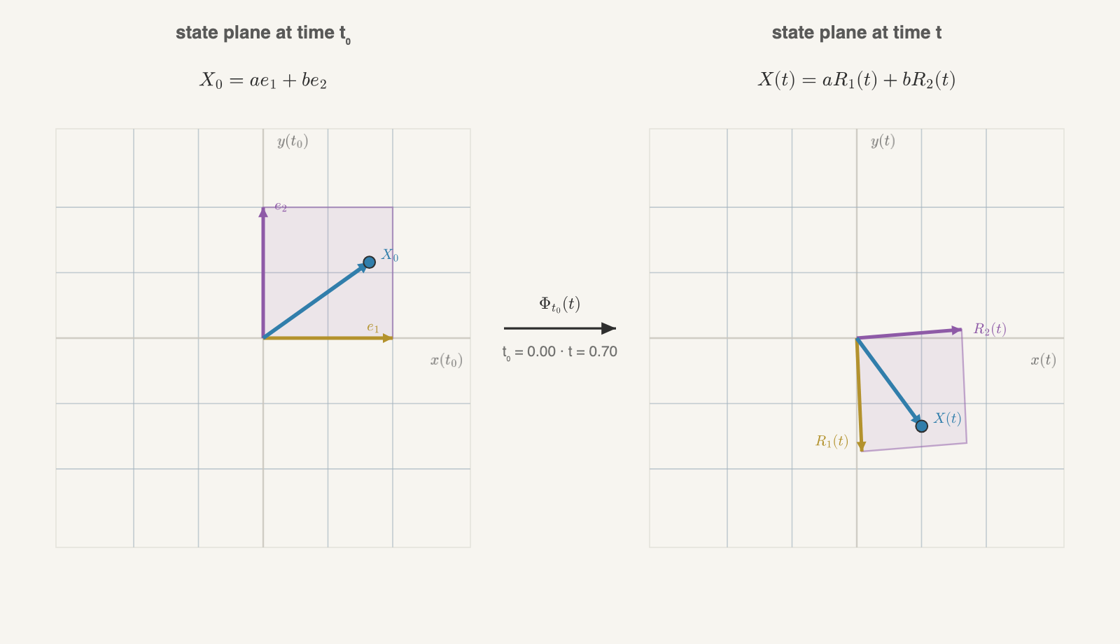
Figure 6.3 For the time-dependent system above, the left panel shows $𝑋 0 = 𝑎 𝑒 1 + 𝑏 𝑒 2$ . The flow map sends the basis vectors to $𝑅 1 (𝑡)$ and $𝑅 2 (𝑡)$ , so the right panel shows $𝑋 (𝑡) = 𝑎 𝑅 1 (𝑡) + 𝑏 𝑅 2 (𝑡)$ . Drag $𝑋 0$ , or change the starting and elapsed times, to compare the two linear combinations.

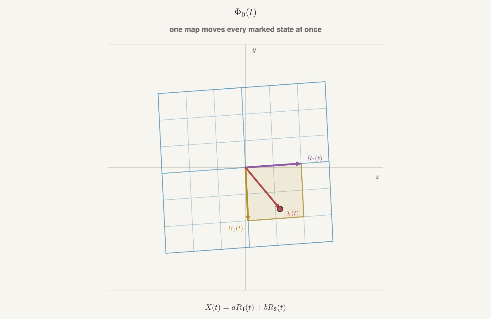
Figure 6.4 The map $Φ 0 (𝑡)$ acts simultaneously on a grid of initial states, the standard basis, the unit square, and one selected state. The coefficients $𝑎, 𝑏$ remain fixed while the basis vectors and selected state move. Each frame displays one linear map at one time.

The starting time matters. For our time-dependent system, numerical integration gives

Φ 0 (1) \approx (- 0.462693 0.632462 - 0.661972 - 0.406010), Φ 1 (2) \approx (- 0.433324 0.699270 - 0.627664 - 0.386833) .

Both maps advance the state by one unit of time, but the coefficient matrix changes during those two intervals. Equal elapsed times need not produce equal evolution maps. This is why we retain $𝑡 0$ in the notation.

We have built the flow matrix out of solutions. Can we describe it by a differential equation of its own? Differentiate column by column:

Φ' 𝑡 0 (𝑡) = (𝑅' 1 (𝑡) \dots 𝑅' 𝑁 (𝑡)) = (𝐴 (𝑡) 𝑅 1 (𝑡) \dots 𝐴 (𝑡) 𝑅 𝑁 (𝑡)) = 𝐴 (𝑡) Φ 𝑡 0 (𝑡) .

Thus all the standard initial value problems fit into one matrix initial value problem:

Φ' 𝑡 0 (𝑡) = 𝐴 (𝑡) Φ 𝑡 0 (𝑡), Φ 𝑡 0 (𝑡 0) = 𝐼 .

A solution of this matrix equation supplies the solution from every initial state by $𝑋 (𝑡) = Φ 𝑡 0 (𝑡) 𝑋 0$ . Numerically, the Euler updates for all the columns can likewise be collected into

̂ Φ 𝑛 + 1 = (𝐼 + ℎ 𝐴 (𝑡 𝑛)) ̂ Φ 𝑛, ̂ Φ 0 = 𝐼,

where $𝑡 𝑛 = 𝑡 0 + 𝑛 ℎ$ . This computes an approximation to the flow matrix one step at a time.

There is still a differential equation hidden in the construction: we obtained the columns by solving from the standard initial states. The original equation gives us $𝐴 (𝑡)$ , which assigns the rate of change at an instant. We want $Φ 𝑡 0 (𝑡)$ , which carries out the resulting evolution over an interval. In the next chapter we specialize to a constant matrix $𝐴$ and ask how to construct that evolution directly from the matrix itself.

Problems

Check Your Understanding

1Determine the dimension

For each homogeneous linear problem below, assume continuous coefficients and equations solved for their highest derivatives. State how many independent pieces of initial data are needed and hence the dimension of the solution space. How many solutions form a basis? List the initial data at $𝑡 = 0$ for the solutions corresponding to the standard basis of the state space.

(a)

$𝑦 ‴ + 𝑎 2 (𝑡) 𝑦 ″ + 𝑎 1 (𝑡) 𝑦' + 𝑎 0 (𝑡) 𝑦 = 0$ .

(b)

A homogeneous first-order system in four unknown functions.

(c)

Two coupled second-order equations for $𝑥 (𝑡)$ and $𝑦 (𝑡)$ . First rewrite the state in first-order form before counting.

Python: Reusing Computed Solutions

2Combine computed solutions

Use the Euler function from Chapter 2 to compute solutions of $𝑦' = 𝑡 𝑦$ from initial values $2$ , $- 1$ , and $5$ on the same time grid.

(a)

Form the array $2 𝑌 2 - 𝑌 - 1$ from the first two computed solutions. Which initial value does this combination have? Compare it point by point with the separately computed solution from that initial value.

(b)

Plot the difference between the combined and directly computed arrays. Is the difference exactly zero, close to zero, or visibly large? Explain why Euler's update itself preserves superposition for this linear equation.

(c)

Repeat the experiment with the logistic equation $𝑦' = 𝑦 (1 - 𝑦 / 10)$ . Plot the combined approximation and the directly computed approximation together, then plot their difference. At what step does the mismatch first appear?