In the last chapter, we computed the matrix exponential for three especially
simple matrices: a diagonal matrix, the rotation matrix 𝐽, and the shear
matrix 𝑁. Their powers followed patterns that let us sum the exponential
series explicitly. Our goal now is to compute the flow of every real
2×2 matrix. Remarkably, those three examples will supply everything
we need.
The key is to choose coordinates in which the matrix becomes simple. We'll
investigate three possibilities: two linearly independent real eigenvectors,
just one independent real eigenvector, and no real eigenvectors. These lead
to diagonal motion, shear, and rotation, with uniform exponential scaling
appearing alongside the latter two. We'll begin with two independent
eigenvectors, where the matrix itself gives us the coordinate directions to
use.
8.1Two Independent Eigenvectors
An eigenvector gives us a direction in which the velocity rule acts simply.
If 𝐴𝑣=𝜆𝑣, then at any state 𝑐𝑣 on the line through 𝑣, the
velocity is
𝐴(𝑐𝑣)=𝑐𝜆𝑣.
It points along the same line, so the motion stays on that line. If we have
two independent eigenvectors, we have two such directions—and those
directions form a basis of the plane.
For example, consider
𝐴=(4123).
Its characteristic polynomial is
det(𝐴−𝜆𝐼)=(4−𝜆)(3−𝜆)−2=𝜆2−7𝜆+10=(𝜆−5)(𝜆−2).
The eigenvalues are 5 and 2. Solving 𝐴𝑣=𝜆𝑣 for each gives the
eigenvectors
𝑣1=(11),𝑣2=(1−2),
with 𝐴𝑣1=5𝑣1 and 𝐴𝑣2=2𝑣2. These vectors are independent, so we can
use them as our coordinate directions. What does the matrix look like in
these coordinates?
In a basis of eigenvectors, applying 𝐴 just multiplies each coordinate by
its eigenvalue. Indeed, if 𝐴𝑣1=𝜆1𝑣1 and 𝐴𝑣2=𝜆2𝑣2, then
𝐴(𝑢𝑣1+𝑤𝑣2)=𝜆1𝑢𝑣1+𝜆2𝑤𝑣2.
The coordinates (𝑢,𝑤) become (𝜆1𝑢,𝜆2𝑤). So in this basis,
the matrix is diagonal:
𝐷=(𝜆100𝜆2).
To relate this to the original matrix, put the eigenvectors in the columns
of 𝑃=(𝑣1𝑣2). Multiplying by 𝑃 converts eigenvector coordinates to
ordinary coordinates:
𝑃(𝑢𝑤)=𝑢𝑣1+𝑤𝑣2.
Because the eigenvectors form a basis, 𝑃 is invertible, and 𝑃−1
converts back. The eigenvector equations give
𝐴𝑃=(𝐴𝑣1𝐴𝑣2)=(𝜆1𝑣1𝜆2𝑣2)=𝑃𝐷,
so
𝐴=𝑃𝐷𝑃−1.
Read from right to left: convert to eigenvector coordinates, multiply each
coordinate by its eigenvalue, and convert back. This is the same linear
transformation 𝐴, expressed using a basis in which its action is simple.
A matrix that admits such a representation is called diagonalizable.
For our example,
𝑃=(111−2),𝐷=(5002).
We have written 𝐴 in terms of a diagonal matrix. How does this help us
compute 𝑒𝑡𝐴?
Substituting 𝐴=𝑃𝐷𝑃−1 into the exponential series gives
𝑒𝑡𝐴=𝐼+𝑡(𝑃𝐷𝑃−1)+𝑡22!(𝑃𝐷𝑃−1)2+𝑡33!(𝑃𝐷𝑃−1)3+⋯.
So we need to compute powers of 𝑃𝐷𝑃−1. When we multiply two copies
together, the middle factors cancel:
(𝑃𝐷𝑃−1)2=𝑃𝐷𝑃−1𝑃𝐷𝑃−1=𝑃𝐷2𝑃−1.
The same cancellation occurs between every pair of consecutive copies, so
(𝑃𝐷𝑃−1)𝑘=𝑃𝐷𝑘𝑃−1.
Only the diagonal matrix needs to be raised to a power! Substituting these
expressions into the series, and writing 𝐼=𝑃𝐼𝑃−1, we get
Nothing in the cancellation required 𝐷 to be diagonal. The same
calculation proves a general result.
Theorem 8.1 (Exponentials in new coordinates). If 𝐴=𝑃𝐶𝑃−1, where 𝑃 is invertible, then
𝑒𝑡𝐴=𝑃𝑒𝑡𝐶𝑃−1.
For a diagonalizable matrix, this gives
𝑒𝑡𝐴=𝑃(𝑒𝜆1𝑡00𝑒𝜆2𝑡)𝑃−1.
Read from right to left, the flow first finds the state's eigenvector
coordinates, multiplies each by its own exponential, and converts back. In
these coordinates, the two components evolve independently.
We can understand this answer directly from the factored form
𝑃𝑒𝑡𝐷𝑃−1. The first step finds the initial state's eigenvector
coordinates:
𝑃−1𝑋0=13(211−1)(2−1)=(11).
So 𝑋0=𝑣1+𝑣2. Each component evolves by its own exponential, giving
𝑋(𝑡)=𝑒5𝑡(11)+𝑒2𝑡(1−2).
This is the same answer, now expressed as motion along the two eigenvector
directions.
The calculation works for any initial state and any eigenvector basis.
Theorem 8.2 (Solutions in an eigenvector basis). Suppose a real 2×2 matrix 𝐴 has two independent real eigenvectors
𝑣1,𝑣2, with eigenvalues 𝜆1,𝜆2. Write the initial state as
𝑋0=𝑐1𝑣1+𝑐2𝑣2.
Then the solution of 𝑋′=𝐴𝑋, 𝑋(0)=𝑋0, is
𝑋(𝑡)=𝑐1𝑒𝜆1𝑡𝑣1+𝑐2𝑒𝜆2𝑡𝑣2.
The same argument works in any dimension: whenever 𝐴 has an eigenvector
basis, each component of the initial state evolves by its corresponding
exponential.
8.1.1The Geometry of Diagonal Flows
The formula
𝑋(𝑡)=𝑐1𝑒𝜆1𝑡𝑣1+𝑐2𝑒𝜆2𝑡𝑣2
lets us read the motion from the eigenvalues. Each component grows, decays,
or stays fixed according to the sign of its eigenvalue.
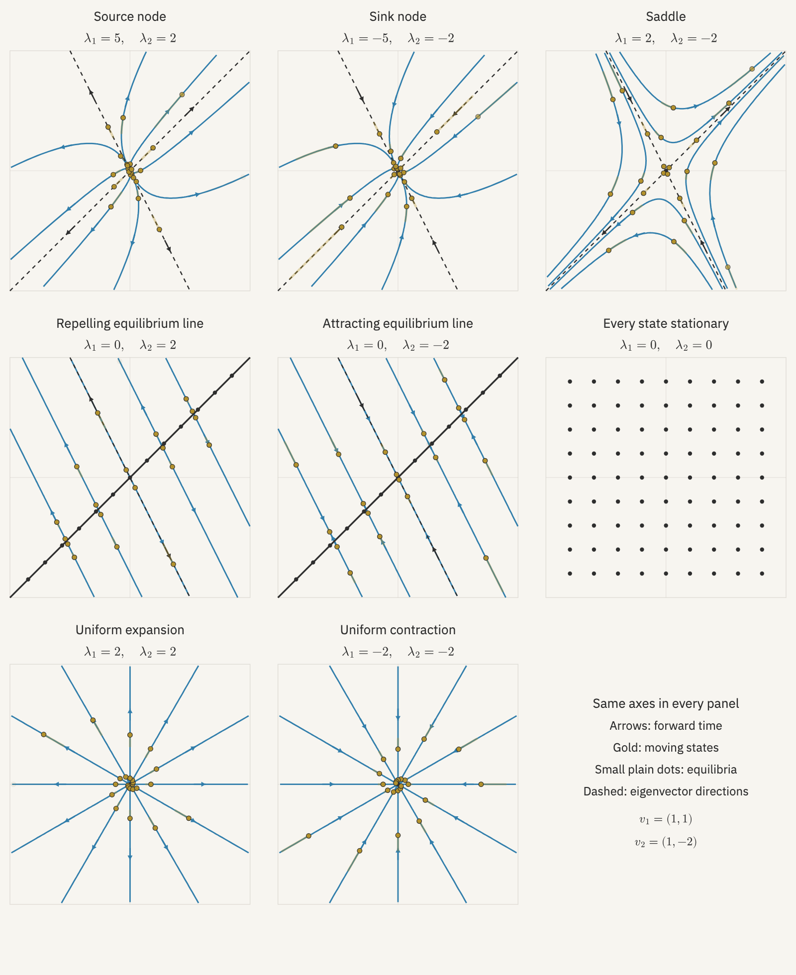
When both eigenvalues are positive, every nonzero state eventually moves
arbitrarily far from the origin: a source node. When both are negative,
every state approaches the origin: a sink node. If the rates differ,
the faster-growing component eventually dominates a source, while the
slower-decaying component dominates a sink—unless that component is absent
from the initial state.
When the eigenvalues have opposite signs, the flow is a saddle. One
eigenvector line attracts states toward the origin; the other repels them.
Trajectories on neither line come in along the attracting direction and
leave along the repelling direction. Only states on the attracting line
approach the origin as 𝑡→∞.
If exactly one eigenvalue is zero, its eigenvector line consists of
equilibria. Every other trajectory runs parallel to the other eigenvector,
approaching the equilibrium line when the nonzero eigenvalue is negative
and moving away when it is positive.
Finally, suppose the two eigenvalues are equal to 𝜆. Since we have
an eigenvector basis, 𝐷=𝜆𝐼, so
𝐴=𝑃(𝜆𝐼)𝑃−1=𝜆𝐼. The flow scales uniformly: every nonzero
state moves outward along its ray when 𝜆>0, and inward when
𝜆<0. When 𝜆=0, 𝐴=0, and every state is stationary.
Figure 8.1 (Draft caption — final wording at prose stage.) Compare the flows as the
two eigenvalues change. The axes and eigenvector directions are the same
in every panel. Arrows show the direction of motion, and small plain dots
mark equilibria. In the live figure, gold dots and short trails follow the
flow while the equilibrium marks stay fixed. When one eigenvalue is zero,
an entire line is stationary;
when both are zero, every state is stationary.
8.2One Independent Eigenvector
Suppose we have an eigenvector 𝑣, with eigenvalue 𝜆, but cannot
find a second independent eigenvector. We can still complete 𝑣 to a
basis: choose any vector 𝑤 not on its line. What does 𝐴 look like in
this basis?
Since 𝐴𝑣=𝜆𝑣, the first column is (𝜆,0). Write
𝐴𝑤=𝑐𝑣+𝜇𝑤 for the second column. Thus, with 𝑃=(𝑣𝑤),
𝑃−1𝐴𝑃=𝐶=(𝜆𝑐0𝜇).
We have made one entry zero, even though we could not diagonalize the
matrix.
The characteristic polynomial of 𝐶 is
det(𝐶−𝑟𝐼)=(𝜆−𝑟)(𝜇−𝑟),
so its eigenvalues are 𝜆 and 𝜇. If they were different, 𝐴
would have two independent eigenvectors. Therefore 𝜇=𝜆. Also,
𝑐≠0: if 𝑐=0, we would have 𝐶=𝜆𝐼, and every direction would
be an eigenvector.
So the matrix must have the form
𝐶=(𝜆𝑐0𝜆)=𝜆𝐼+𝑐𝑁,𝑁=(0100).
There is our second familiar matrix! In these coordinates, the velocity
rule combines uniform scaling with the shear from Chapter 7.
Since 𝜆𝐼 commutes with 𝑐𝑁, we can exponentiate the two parts
separately:
𝑒𝑡𝐶=𝑒𝑡(𝜆𝐼+𝑐𝑁)=𝑒𝜆𝑡𝑒𝑐𝑡𝑁.
And 𝑁2=0, so the second exponential stops after two terms:
𝑒𝑐𝑡𝑁=𝐼+𝑐𝑡𝑁=(1𝑐𝑡01).
Our change-of-coordinates theorem now gives
𝑒𝑡𝐴=𝑃𝑒𝑡𝐶𝑃−1=𝑒𝜆𝑡𝑃(1𝑐𝑡01)𝑃−1.
Multiplying by 𝑋0 gives the solution from any initial state.
The shear contributes the factor 𝑡, and the uniform scaling multiplies
it by 𝑒𝜆𝑡. Since 𝑃 and 𝑃−1 are constant matrices, every
entry of 𝑒𝑡𝐴 is a combination of 𝑒𝜆𝑡 and 𝑡𝑒𝜆𝑡.
So each unknown has the form
𝑥(𝑡)=(𝑎+𝑏𝑡)𝑒𝜆𝑡.
The extra factor of 𝑡 comes from shear.
Example 8.3 (Computing a flow with one eigenvector direction). Consider
𝐴=(11−13).
Its characteristic polynomial is
det(𝐴−𝜆𝐼)=(1−𝜆)(3−𝜆)+1=(𝜆−2)2.
The only eigenvalue is 2, and solving (𝐴−2𝐼)𝑣=0 gives the line of
eigenvectors 𝑣=(1,1). Complete this to a basis by choosing 𝑤=(0,1). Then
𝐴𝑣=2𝑣,𝐴𝑤=(1,3)=𝑣+2𝑤.
Thus
𝑃=(1011),𝐶=𝑃−1𝐴𝑃=(2102)=2𝐼+𝑁.
The scaling rate is 2, and the shear rate is 1. Our formula gives
𝑒𝑡𝐴=𝑒2𝑡(1011)(1𝑡01)(10−11)=𝑒2𝑡(1−𝑡𝑡−𝑡1+𝑡).
So the solution from 𝑋0=(𝑥0,𝑦0) is
𝑋(𝑡)=𝑒2𝑡((1−𝑡)𝑥0+𝑡𝑦0−𝑡𝑥0+(1+𝑡)𝑦0).
For instance, starting from 𝑋0=(0,1) gives
𝑥(𝑡)=𝑡𝑒2𝑡,𝑦(𝑡)=(1+𝑡)𝑒2𝑡.
Starting instead from the eigenvector 𝑋0=(1,1) gives
𝑥(𝑡)=𝑦(𝑡)=𝑒2𝑡: on the invariant line, the shear term disappears.
8.2.1The Geometry of Shear Flows
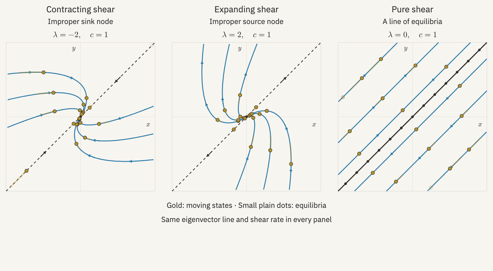
The sign of 𝜆 determines whether the scaling eventually overcomes
the shear. When 𝜆<0, both 𝑒𝜆𝑡 and 𝑡𝑒𝜆𝑡 tend
to zero, so every state approaches the origin. When 𝜆>0, every
nonzero state eventually moves arbitrarily far away. These are again sink
and source nodes, but now there is only one eigenvector direction. They are
called improper nodes.
For the sink, trajectories off the eigenvector line approach the origin
tangent to that line. The source has the time-reversed picture:
trajectories leave the origin tangent to the eigenvector line, then bend
away. States on the line remain on it and move purely exponentially.
When 𝜆=0, only the shear remains. Every state on the eigenvector
line is an equilibrium, while states off it move at constant velocity
along parallel lines. Unlike the diagonalizable zero-eigenvalue case,
these trajectories neither approach nor leave the equilibrium line; they
slide alongside it.
Figure 8.2 Compare the same shear with exponential contraction, exponential expansion,
and no scaling. The eigenvector line is the same in all three panels.
Gold dots and short trails follow moving states; the plain dots on the
pure-shear panel mark a whole line of equilibria.
(Draft caption — final wording at prose stage.)
8.3No Real Eigenvectors
What if there are no real eigenvectors at all? Then there are no invariant
lines to use as coordinate directions. We already know one matrix like
this:
𝐽=(01−10).
For every nonzero state 𝑋, the velocity 𝐽𝑋 is perpendicular to 𝑋, so
it cannot be a multiple of 𝑋. Its flow is the rotation we computed in
Chapter 7:
𝑒𝑡𝐽=(cos𝑡sin𝑡−sin𝑡cos𝑡).
What happens if we multiply 𝐽 by a number 𝜔>0? Since 𝐽2=−𝐼,
its powers alternate between multiples of 𝐼 and 𝐽. Grouping the even
and odd powers in the exponential series gives
This is a clockwise rotation through angle 𝜔𝑡: multiplying 𝐽 by
𝜔 multiplies the angular speed by 𝜔.
Adding 𝑎𝐼 adds a velocity 𝑎𝑋 along the ray through each state. As with
shear, the two parts commute, so
𝑒𝑡(𝑎𝐼+𝜔𝐽)=𝑒𝑎𝑡𝑒𝜔𝑡𝐽=𝑒𝑎𝑡(cos𝜔𝑡sin𝜔𝑡−sin𝜔𝑡cos𝜔𝑡).
The flow rotates clockwise at angular speed 𝜔, while scaling
lengths by 𝑒𝑎𝑡.
We will show that every real 2×2 matrix with no real eigenvectors
has this form in a suitable basis. As in the previous cases, finding that
basis will reduce the exponential to a computation we already know.
Before finding the basis, we can determine what 𝑎 and 𝜔 would have
to be. Changing coordinates preserves the characteristic polynomial:
det(𝑃−1𝐴𝑃−𝜆𝐼)=det(𝑃−1(𝐴−𝜆𝐼)𝑃)=det(𝐴−𝜆𝐼).
For the matrix we want,
det(𝑎𝐼+𝜔𝐽−𝜆𝐼)=det(𝑎−𝜆𝜔−𝜔𝑎−𝜆)=(𝑎−𝜆)2+𝜔2.
Expanding and comparing with the characteristic polynomial of 𝐴 gives
𝜆2−2𝑎𝜆+𝑎2+𝜔2=𝜆2−(tr𝐴)𝜆+det𝐴.
The coefficients must match, so
𝑎=tr𝐴2,𝜔2=det𝐴−𝑎2.
Since 𝐴 has no real eigenvalues, its characteristic polynomial has
negative discriminant:
(tr𝐴)2−4det𝐴<0.
Thus det𝐴−𝑎2>0, and we can take 𝜔=√det𝐴−𝑎2.
These are the only possible values. It remains to show that a basis giving
the desired matrix actually exists. First remove the scaling part: write
𝐴=𝑎𝐼+𝐵,𝐵=𝐴−𝑎𝐼.
The commuting law gives
𝑒𝑡𝐴=𝑒𝑎𝑡𝑒𝑡𝐵.
So our remaining task is to find a basis in which 𝐵 becomes 𝜔𝐽.
The key property of 𝐽 is 𝐽2=−𝐼. For 𝜔𝐽, this becomes
(𝜔𝐽)2=−𝜔2𝐼. Let's check whether 𝐵 satisfies the same
identity.
Since 𝑎 is half the trace of 𝐴, the matrix 𝐵=𝐴−𝑎𝐼 has trace zero. Its
diagonal entries are therefore negatives of one another, and direct
multiplication gives
𝐵=(𝑝𝑞𝑟−𝑝),𝐵2=(𝑝2+𝑞𝑟00𝑝2+𝑞𝑟)=−(det𝐵)𝐼.
To find det𝐵, evaluate the characteristic polynomial of 𝐴 at
𝜆=𝑎:
det𝐵=det(𝐴−𝑎𝐼)=𝑎2−(tr𝐴)𝑎+det𝐴=det𝐴−𝑎2=𝜔2.
Thus
𝐵2=−𝜔2𝐼.
Now we can construct the basis. The matrix 𝜔𝐽 sends 𝑒1 to
−𝜔𝑒2 and 𝑒2 to 𝜔𝑒1. We want vectors 𝑣,𝑤 on which
𝐵 acts in exactly this way:
𝐵𝑣=−𝜔𝑤,𝐵𝑤=𝜔𝑣.
Choose any nonzero 𝑣. The first equation tells us to set
𝑤=−1𝜔𝐵𝑣.
The second then follows from the identity we just proved:
𝐵𝑤=−1𝜔𝐵2𝑣=𝜔𝑣.
These vectors are independent. If 𝑤 were a multiple of 𝑣, then
𝐵𝑣=−𝜔𝑤 would also be a multiple of 𝑣, making 𝑣 an eigenvector
of both 𝐵 and 𝐴=𝑎𝐼+𝐵. But 𝐴 has no real eigenvectors.
So 𝑣,𝑤 form a basis. With 𝑃=(𝑣𝑤), the two equations above say
𝐵𝑃=𝑃(𝜔𝐽),
and consequently
𝑃−1𝐴𝑃=𝑎𝐼+𝑃−1𝐵𝑃=𝑎𝐼+𝜔𝐽.
We have found the desired coordinates.
Theorem 8.4 (Rotation coordinates). Let 𝐴 be a real 2×2 matrix with no real eigenvectors, and set
𝑎=tr𝐴2,𝜔=√det𝐴−𝑎2,𝐵=𝐴−𝑎𝐼.
Choose any nonzero vector 𝑣, let 𝑤=−𝐵𝑣/𝜔, and set 𝑃=(𝑣𝑤).
Then 𝑃 is invertible and
𝑃−1𝐴𝑃=𝑎𝐼+𝜔𝐽.
Our change-of-coordinates theorem now gives the flow:
𝑒𝑡𝐴=𝑒𝑎𝑡𝑃(cos(𝜔𝑡)sin(𝜔𝑡)−sin(𝜔𝑡)cos(𝜔𝑡))𝑃−1.
As before, multiplying by 𝑋0 gives the solution from any initial state.
Since 𝑃 and 𝑃−1 are constant, each unknown is a combination of
𝑒𝑎𝑡cos(𝜔𝑡) and 𝑒𝑎𝑡sin(𝜔𝑡).
There is also a convenient way to write the flow directly in terms of 𝐵.
We proved that 𝐵=𝑃(𝜔𝐽)𝑃−1, so 𝑃𝐽𝑃−1=𝐵/𝜔. Therefore
Both unknowns oscillate with an exponentially decaying amplitude, while
the state spirals toward the origin.
8.3.1The Geometry of Rotation Flows
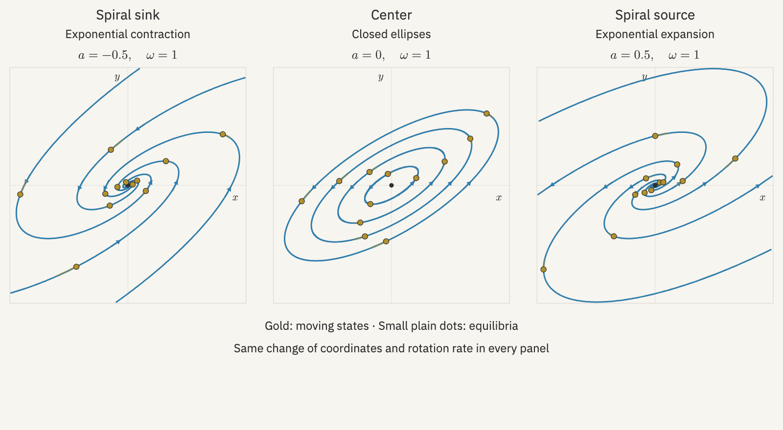
The sign of 𝑎 determines what happens as the states turn. When 𝑎<0,
the factor 𝑒𝑎𝑡 decays, and every nonzero state spirals toward the
origin: a spiral sink. When 𝑎>0, that factor grows, and every nonzero
state spirals outward: a spiral source.
When 𝑎=0, there is no expansion or contraction. In rotation coordinates,
states travel around circles. The change of coordinates 𝑃 maps these
circles to ellipses, so every nonzero trajectory in the original
coordinates is a closed ellipse. This flow is called a center. States
keep circling without approaching the origin or escaping to infinity.
In all three cases, the origin is the only equilibrium. The parameter
𝜔 determines the time for one full turn, 2𝜋/𝜔. The angular
speed is constant in rotation coordinates, though it need not be constant
in the original coordinates.
Figure 8.3 Keep the change of coordinates from the preceding example and 𝜔=1,
and vary only the scaling rate 𝑎. Gold dots and short trails follow
states spiraling inward, circulating around closed ellipses, or spiraling
outward. The origin remains fixed in all three panels.
(Draft caption — final wording at prose stage.)
8.4Trace and Determinant
We have now computed the flow of every real 2×2 matrix. Two
independent eigenvectors give diagonal motion, one gives shear with
scaling, and none gives rotation with scaling. We can organize these
possibilities in a single picture using the characteristic polynomial:
det(𝐴−𝜆𝐼)=𝜆2−(tr𝐴)𝜆+det𝐴.
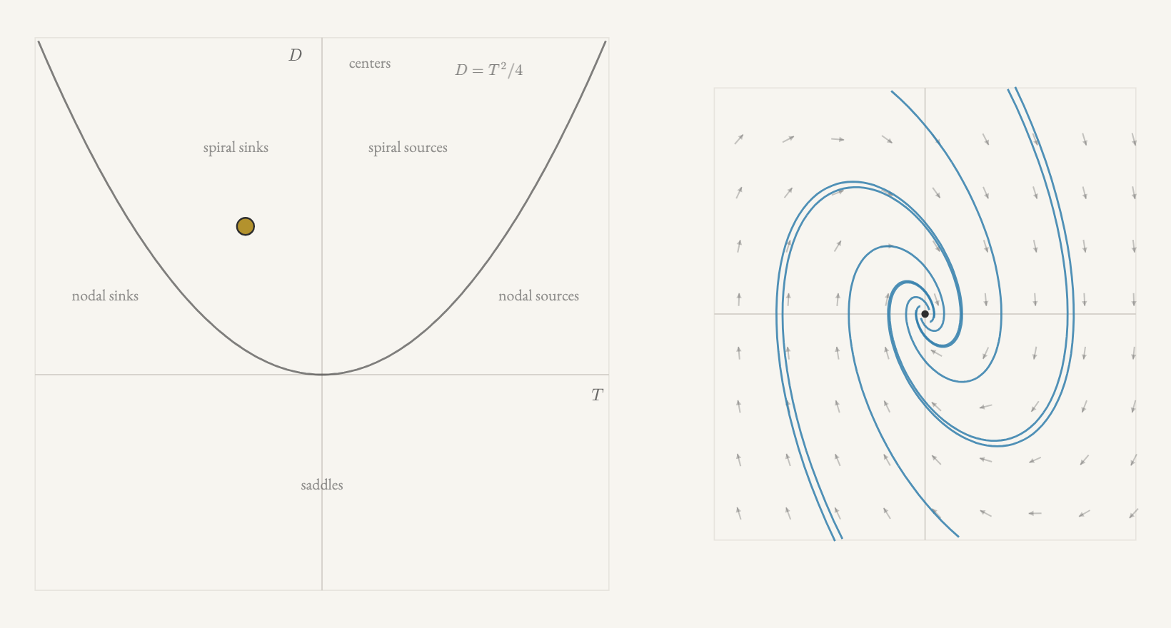
Its coefficients are just the trace and determinant. So draw a plane with
tr𝐴 on the horizontal axis and det𝐴 on the vertical
axis. Each matrix determines a point in this plane.
The discriminant
(tr𝐴)2−4det𝐴
tells us whether the characteristic polynomial has two distinct real
roots, a repeated root, or no real roots. The boundary is therefore the
parabola
det𝐴=14(tr𝐴)2.
Below it, there are two distinct real eigenvalues, so the matrix is
diagonalizable. Above it, there are no real eigenvalues, so the flow
combines rotation and scaling. On the parabola, the eigenvalue is
repeated: the flow either scales uniformly or combines shear with
scaling. Trace and determinant alone cannot distinguish those last two
possibilities.
To distinguish sources from sinks and saddles, recall that
𝜆1+𝜆2=tr𝐴,𝜆1𝜆2=det𝐴.
Below the horizontal axis, the determinant is negative, so the eigenvalues
have opposite signs. This entire region consists of saddles.
Between the horizontal axis and the parabola, the eigenvalues are real and
have positive product, so they have the same sign. Their sum tells us
which sign: negative trace gives a sink node, and positive trace gives a
source node.
Above the parabola, the flow combines rotation with scaling at rate
𝑎=12tr𝐴. Negative trace gives a spiral sink,
positive trace gives a spiral source, and zero trace gives a center.
The boundaries contain the remaining cases. On the parabola, the repeated
eigenvalue is 𝜆=12tr𝐴, so negative trace gives
contraction and positive trace gives expansion, either uniformly or with
shear. On the horizontal axis away from (0,0), one eigenvalue is zero and
the other equals the trace. There is a line of equilibria, attracting when
the trace is negative and repelling when it is positive.
At (0,0) in the diagram, both eigenvalues are zero. If 𝐴=0, every state
is stationary. Otherwise, the flow is a pure shear. This is another place
where we must inspect the matrix itself to distinguish two flows with the
same trace and determinant.
Figure 8.4 Move the point in the trace–determinant plane to see a flow with those
values. Gold dots and short trails follow moving states; plain dots mark
equilibria. On the parabola, switch between shear and uniform scaling
without moving the parameter point. At (0,0), compare pure shear with
the zero matrix: the same trace and determinant can describe different
flows.
(Draft caption — final wording at prose stage.)
8.5The Damped Spring
The damped spring has equation
𝑥″+𝑏𝑥′+𝑘𝑥=0,
where the mass is normalized to 1, 𝑘>0 measures the spring's strength,
and 𝑏≥0 measures the damping. With 𝑣=𝑥′, this becomes the linear
system
(𝑥𝑣)′=(01−𝑘−𝑏)(𝑥𝑣).
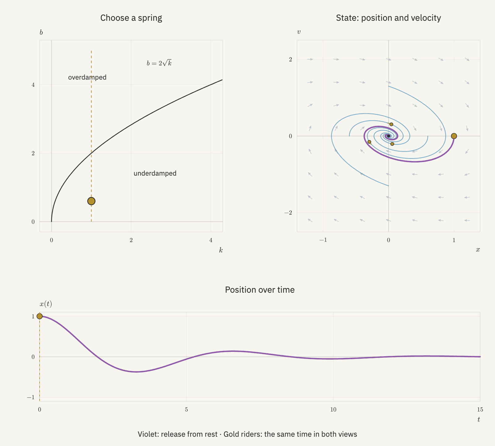
A pair (𝑘,𝑏) specifies a spring system: how strong the spring is and how
much friction opposes its motion. Draw 𝑘 on the horizontal axis and 𝑏
on the vertical axis. Each point chooses a system; the other two plots
show its motion as a trajectory in the (𝑥,𝑣)-plane and as a graph of
position over time.
The system's matrix has trace −𝑏 and determinant 𝑘, so the discriminant
is
(tr𝐴)2−4det𝐴=𝑏2−4𝑘.
The boundary between real and nonreal eigenvalues is therefore the curve
𝑏=2√𝑘.
We can explore all the damping cases by fixing 𝑘 and increasing 𝑏:
moving straight upward in the parameter plane.
Begin with no friction. At 𝑏=0, the flow is a center. The state travels
around a closed ellipse in the (𝑥,𝑣)-plane: displacement becomes
velocity, then velocity becomes displacement again, and the motion
repeats. The graph of 𝑥(𝑡) shows oscillations of constant amplitude.
Now increase 𝑏. Below the curve 𝑏=2√𝑘, the flow is a spiral sink.
The state still turns around the origin, but each turn brings it closer
to (0,0). In the displacement graph, the spring continues to swing
through equilibrium, with smaller and smaller excursions. This is
underdamping. Our rotation calculation gives
𝑎=−𝑏2,𝜔=√𝑘−𝑏24.
Increasing the damping therefore does two things: it makes the exponential
envelope decay faster, and it slows the oscillations.
At 𝑏=2√𝑘, we reach the boundary and 𝜔 reaches zero.
This is critical damping. Recall what happened here in Chapter 6. The
two exponential solutions collapsed to the same function 𝑒−𝑏𝑡/2. The
oscillating guesses also failed to supply a second solution: the cosine
became 1, and the sine became 0. Yet we knew that the solution space
had dimension two. Multiplying the exponential by 𝑡 gave the missing
solution—but why should that work?
Now we can see what those guesses were missing. At critical damping, the
matrix has the repeated eigenvalue 𝜆=−𝑏/2. It cannot be
𝜆𝐼, because
𝐴=(01−𝑘−𝑏)
has a nonzero off-diagonal entry. So there is only one eigenvector
direction. Motion along that direction gives the exponential we already
found. To describe motion from other initial states, we need the shear.
In a suitable basis, the flow is
𝑒−𝑏𝑡/2(1𝑐𝑡01).
The second direction contributes motion along the first through the entry
𝑐𝑡. After multiplying by the contraction factor and converting back,
the position has the form
𝑥(𝑡)=(𝑐1+𝑐2𝑡)𝑒−𝑏𝑡/2.
The solution space never lost its second dimension. What we lost was a
second eigenvector direction; shear supplies the motion that a second pure
exponential could no longer describe.
Increase 𝑏 further, and the point moves above the curve 𝑏=2√𝑘.
There are again two independent eigenvector directions,
both with negative eigenvalues. The state approaches the origin without
spiraling, and 𝑥(𝑡) is a combination of two decaying exponentials. This
is overdamping. In the figure, the spring released from rest returns
without crossing equilibrium. With strong damping, its final approach
becomes slow: friction suppresses the oscillation, but also impedes the
return.
Figure 8.5 Choose a spring by dragging the point (𝑘,𝑏). Hold 𝑘 fixed and increase
𝑏 to move from undamped oscillation through underdamping, critical
damping, and overdamping. The violet curves show the spring released from
rest at 𝑥=1; matching gold dots show its state and position at the same
time.
Problems
1Solving 𝑥′=𝑥+2𝑦,𝑦′=3𝑥+2𝑦
Consider the system
𝑥′=𝑥+2𝑦,𝑦′=3𝑥+2𝑦.
(a)
Decide which case this system falls into: two independent real
eigenvectors, one, or none.
(b)
Find the solution with initial condition 𝑥(0)=𝑥0, 𝑦(0)=𝑦0. Then
find the solution with 𝑥(0)=1, 𝑦(0)=4.
2Solving 𝑥′=𝑥−4𝑦,𝑦′=2𝑥−3𝑦
Consider the system
𝑥′=𝑥−4𝑦,𝑦′=2𝑥−3𝑦.
(a)
Decide which case this system falls into: two independent real
eigenvectors, one, or none.
(b)
Find the solution with initial condition 𝑥(0)=𝑥0, 𝑦(0)=𝑦0. Then
find the solution with 𝑥(0)=1, 𝑦(0)=1.
3Solving 𝑥′=−𝑥−4𝑦,𝑦′=𝑥−5𝑦
Consider the system
𝑥′=−𝑥−4𝑦,𝑦′=𝑥−5𝑦.
(a)
Decide which case this system falls into: two independent real
eigenvectors, one, or none.
(b)
Find the solution with initial condition 𝑥(0)=𝑥0, 𝑦(0)=𝑦0. Then
find the solution with 𝑥(0)=3, 𝑦(0)=1.
4What the trace measures
The eigenvalues tell us how a flow scales its eigenvector directions.
In this problem, we investigate what they tell us about area.
(a)
Return to the system 𝑥′=𝑥+2𝑦,𝑦′=3𝑥+2𝑦 from Solving 𝑥′=𝑥+2𝑦,𝑦′=3𝑥+2𝑦. Consider the parallelogram whose
sides are the eigenvectors
𝑣1=(2,3),𝑣2=(1,−1).
Under the flow, by what factor does each side scale after time 𝑡?
By what factor does the area change? Explain why the area grows even
though one side contracts.
(b)
A linear map with matrix 𝑀 multiplies areas by |det𝑀|. For the
system 𝑋′=𝐴𝑋, the flow matrix is 𝑒𝑡𝐴, so its determinant tells
us how the flow changes area.
Suppose 𝐴 has two independent real eigenvectors. Show that
det(𝑒𝑡𝐴)=𝑒𝑡tr𝐴.
(Hint: use diagonalization and the identity det(𝑋𝑌)=det(𝑋)det(𝑌)
to simplify your calculation.)
(c)
Give an example of a system 𝑋′=𝐴𝑋 whose flow preserves area but has
trajectories that travel arbitrarily far from the origin. You may
choose 𝐴 to be diagonal. Explain how your example has both
properties.
The formula in part (b) also holds when 𝐴 has only one independent
real eigenvector or none. For every real 2×2 matrix, the trace
determines the area factor: positive trace gives exponential area
growth, negative trace gives exponential area decay, and zero trace
gives area preservation.
5How far can a sink carry a state?
Consider the family of systems
𝑥′=−𝑥+𝑐𝑦,𝑦′=−2𝑦,
where 𝑐>0 is a constant.
(a)
Find the eigenvalues and classify the flow. Explain why every solution
approaches the origin as 𝑡→∞, no matter how large 𝑐 is.
(b)
Now follow the solution starting at
𝑥(0)=0,𝑦(0)=1.
You may use the eigenvectors (1,0) and (𝑐,−1). Write the initial
state as a combination of these vectors, then find 𝑥(𝑡) and 𝑦(𝑡).
When does 𝑥(𝑡) reach its largest value for 𝑡≥0? How does that
value depend on 𝑐? Use your answer to choose a system whose
trajectory starts one unit from the origin, travels more than 100
units away, and eventually returns to the origin.
Every system in this family is a sink, yet you have shown that a state
can travel far from the origin before returning. Being a sink describes
what happens in the long run; it does not require trajectories to move
steadily closer to the origin.
6Classify the flow
For each system below, decide what kind of flow it has. Is it a
source, where states move away from the origin in both eigenvector
directions? A sink, where states move toward the origin in both? A
saddle, with one direction in and one out? Or a spiral? If it's a
spiral, does it spiral inward or outward?
(a)
𝑥′=𝑦,𝑦′=−2𝑥−3𝑦
(b)
𝑥′=𝑥+3𝑦,𝑦′=2𝑥
(c)
𝑥′=𝑥−𝑦,𝑦′=𝑥+𝑦
(d)
𝑥′=−𝑥−2𝑦,𝑦′=𝑥−𝑦
(e)
𝑥′=4𝑥−𝑦,𝑦′=2𝑥+𝑦
(f)
𝑥′=2𝑥+5𝑦,𝑦′=𝑥−2𝑦
(g)
Two of these systems have positive trace and positive determinant, but only
one of them is a spiral. What decides the difference?
7Design a flow
So far we have started from a matrix and found its flow. In this problem,
we go the other way: we start from a description of the motion and find a
matrix that produces it.
(a)
Find a matrix 𝐴 whose flow is a saddle with these invariant lines. States
on the line 𝑦=𝑥 approach the origin, scaling by 𝑒−𝑡. States on the
line 𝑦=−𝑥 move away from it, scaling by 𝑒2𝑡.
(b)
Find a matrix 𝐴 whose flow spirals clockwise into the origin, with this
timing. After 𝜋 units of time, every state is back on the ray it started
on, at 𝑒−𝜋 times its starting distance.
(c)
Find a damped spring 𝑥″+𝑏𝑥′+𝑘𝑥=0 whose flow in the (𝑥,𝑣)-plane has the
same timing as in part (b). Explain why the trace and determinant are
enough to decide this.
8Can a heavily damped spring pass through equilibrium?
In the chapter's damped-spring figure, a critically damped or overdamped
spring released from rest returns to equilibrium without ever crossing it.
What if we give the mass a push toward equilibrium instead? In this
problem, the mass starts at 𝑥(0)=1 with velocity 𝑥′(0)=𝑣0. It passes
through equilibrium if 𝑥(𝑡)=0 at some time 𝑡>0.
(a)
The spring 𝑥″+2𝑥′+𝑥=0 is critically damped. Find its solution with
𝑥(0)=1 and 𝑥′(0)=𝑣0.
(b)
For which values of 𝑣0 does this spring pass through equilibrium? How
many times can it do so?
(c)
The spring 𝑥″+3𝑥′+2𝑥=0 is overdamped. Show that a nonzero solution can
pass through equilibrium at most once. For which values of 𝑣0 does it
pass through equilibrium?
(d)
Write each spring as a system 𝑋′=𝐴𝑋 with state 𝑋=(𝑥,𝑣). In part (b),
the spring passes through equilibrium when 𝑣0<−1 but not when 𝑣0=−1.
Show that the starting state (1,−1) is an eigenvector of the matrix for
𝑥″+2𝑥′+𝑥=0. In part (c), the cutoff is 𝑣0=−2. Show that the starting
state (1,−2) is an eigenvector of the matrix for 𝑥″+3𝑥′+2𝑥=0. Then
explain why a solution that starts on an eigenvector line never passes
through equilibrium.
9Sliding to a stop
Give an object a push along a table and let it slide. Suppose the only
horizontal force is the drag from Chapter 4, which opposes the velocity
with strength proportional to speed. With 𝑚=1 and 𝑏=2, the object's
position satisfies
𝑥″+2𝑥′=0.
This is a damped spring with no spring: nothing pulls the object back toward
any particular position.
(a)
Write the equation as a system 𝑋′=𝐴𝑋 with state 𝑋=(𝑥,𝑣). Find the trace
and determinant of 𝐴. Where does 𝐴 lie in the trace–determinant plane,
and what kind of flow does that predict?
(b)
Find the eigenvalues and eigenvectors of 𝐴. Which states are equilibria?
Explain physically why an object at rest stays put.
(c)
Find the solution with 𝑥(0)=𝑥0 and 𝑣(0)=𝑣0. Where does the object come
to rest? How far does it slide after being pushed with velocity 𝑣0?
(d)
Show that every trajectory in the (𝑥,𝑣)-plane lies on a line parallel to
an eigenvector. Sketch several trajectories, and mark the equilibrium that
each one approaches.
10Romeo and Juliet
Steven Strogatz once suggested teaching linear systems through a love
affair. Let 𝑅(𝑡) measure Romeo's love for Juliet and 𝐽(𝑡) Juliet's love
for Romeo, with negative values meaning dislike. The model is a fiction,
but the signs in it have meaning. Suppose both lovers follow the same rule:
𝑅′=𝑎𝑅+𝑏𝐽,𝐽′=𝑏𝑅+𝑎𝐽,𝑎<0<𝑏.
(a)
Explain what 𝑎<0 and 𝑏>0 say about how each lover's feelings change.
Why might we call these lovers cautious?
(b)
Show that (1,1) and (1,−1) are eigenvectors, and find their
eigenvalues.
(c)
Suppose caution outweighs responsiveness: 𝑏<|𝑎|. Classify the flow, and
describe what eventually happens to the affair, whatever the initial
feelings.
(d)
Now suppose 𝑏>|𝑎|. Classify the flow. Show that the long-run outcome
depends only on the sign of 𝑅(0)+𝐽(0), and describe both outcomes. What
happens if 𝑅(0)+𝐽(0)=0?
11More flows to compute
For each system, find the flow 𝑒𝑡𝐴 and the solution from the given
initial state. Then classify the flow and describe the motion.
(a)
𝑥′=2𝑥+𝑦,𝑦′=𝑥+2𝑦, starting from (2,0).
(b)
𝑥′=−𝑦,𝑦′=𝑥+2𝑦, starting from (1,0).
(c)
𝑥′=𝑥+2𝑦,𝑦′=−𝑥−𝑦, starting from (1,0). Show that this solution
stays on the ellipse (𝑥+𝑦)2+𝑦2=1.
12True or false?
Each statement below is about a real 2×2 matrix 𝐴 and the flow of
𝑋′=𝐴𝑋. Decide whether it is true or false. If it is true, explain why. If
it is false, give a matrix for which it fails.
(a)
If tr𝐴=0, the flow is a center.
(b)
If every entry of 𝐴 is negative, the flow is a sink.
(c)
If the flow is a sink, every state moves steadily closer to the origin.
(d)
If 𝐴 has a repeated eigenvalue, it has only one independent eigenvector.