Over the last part of the book, we learned to understand every constant
linear system 𝑋′=𝐴𝑋. A single matrix decides the velocity at every
state, and the matrix exponential 𝑒𝑡𝐴 carries every initial state
forward at once. In good coordinates, the flow breaks into simple
pieces: lines that scale, planes that rotate while scaling, and shears.
Once we have found these pieces, we know what every solution does, from
every initial state and for all time.
All of this depends on linearity. Scaling an initial state scales its
solution, and adding initial states adds their solutions. So a linear
flow looks the same at every scale: the picture near the origin,
magnified, is the picture everywhere. But most of the models we built in
chapter 4 aren't linear. Logistic growth contains a 𝑃2 term, because
a crowded population limits its own growth. The Lotka--Volterra and SIR
equations contain products like 𝐻𝐿 and 𝑆𝐼, because populations change
when they meet. We already saw what this costs in chapter 5:
for 𝑦′=𝑦2, doubling the solution from 𝑦(0)=1 does not give the
solution from 𝑦(0)=2. Without linearity there is no matrix exponential,
and usually no formula at all.
So in this chapter we take a tour. We won't develop new methods yet.
Instead we will look at a few nonlinear systems, each chosen to show one
kind of behavior that no linear flow can have, and compare it with what
we know from the linear world.
11.1Two Resting Places
A linear system 𝑋′=𝐴𝑋 always has the origin as an equilibrium. If it
has another one, 𝑋0, then 𝐴(𝑐𝑋0)=𝑐𝐴𝑋0=0 for every number 𝑐, so
every state on the line through 𝑋0 is an equilibrium too. So a linear
system has either exactly one equilibrium or infinitely many, filling a
line, a plane, or a larger subspace. Its type is the same everywhere. The spring 𝑥″=−𝑥 is the
familiar example: the origin is a center, and wherever we release the
mass, it swings back and forth around 𝑥=0.
Let's replace the spring's force −𝑥 with a nonlinear one:
𝑥″=𝑥−𝑥3.
The force 𝑥−𝑥3=𝑥(1−𝑥2) pushes the mass away from 0 and toward 1
or −1. With 𝑣=𝑥′, the system 𝑥′=𝑣, 𝑣′=𝑥−𝑥3 has three
equilibria: (−1,0), (0,0), and (1,0).
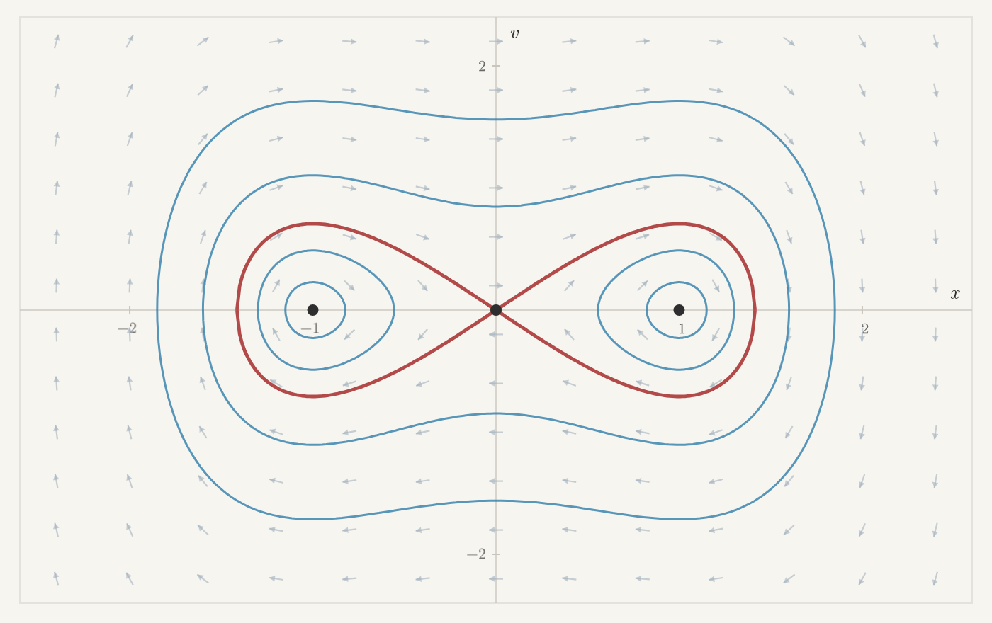
Figure 11.1 Trajectories of 𝑥′=𝑣, 𝑣′=𝑥−𝑥3. The red figure-eight passes through
the equilibrium (0,0). Click to release a state and follow it.
Near (1,0) and (−1,0), states go around closed loops, like a center.
Near (0,0), they come in along one direction and leave along another,
like a saddle. So one system has three separate equilibria, of two
different types. A linear system can have one equilibrium or infinitely
many, but never three.
Something else happens at the saddle. In a linear saddle, the states that
approach the origin lie on one line, and the states that leave it lie on
another. No solution does both: every piece of a linear solution grows or
shrinks like 𝑒𝜆𝑡, and an exponential can't shrink both
forward and backward in time. Now follow the right loop of the red
figure-eight. A state on it leaves the saddle, swings out to 𝑥=√2,
and comes back toward the saddle. A mass released at rest from
𝑥=√2 has exactly enough energy to climb back to the top of the hump
at 0. It creeps up more and more slowly and never quite arrives. Run
backward in time, it came from the top too. So this one solution
approaches the saddle in both directions of time, which no linear
solution can do.
Now add drag. For the linear spring 𝑥″=−𝑥−𝑐𝑥′, the center becomes a
sink: wherever we release the mass, it comes to rest at 𝑥=0. Add the
same drag to the double well:
𝑥″=𝑥−𝑥3−𝑐𝑥′,𝑐>0.
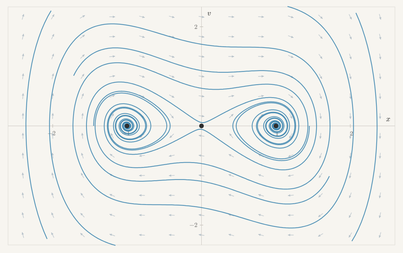
Figure 11.2 Trajectories of 𝑥′=𝑣, 𝑣′=𝑥−𝑥3−14𝑣. Click to release a state
and follow it.
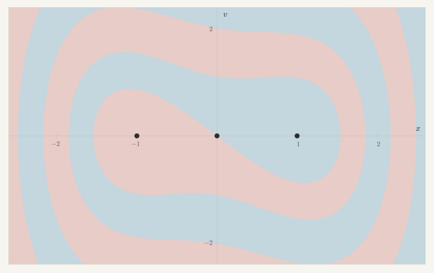
Figure 11.3 Each initial state colored by where it comes to rest: blue for (1,0),
red for (−1,0). Click to release a state and watch it settle. Move
the slider to zoom out.
Near (1,0) and (−1,0), states now spiral inward like a spiral sink,
and (0,0) is still a saddle. Neither sink attracts every state. Each
gets only part of the plane, and the two parts wind around each other in
bands: a mass released farther out swings through the middle more times
before the drag traps it, so its final resting place switches back and
forth.
Near the edge between two colors, a small change in the initial state
changes where the mass comes to rest. Release it at rest from 𝑥=2.164
and from 𝑥=2.174. These states start 0.01 apart, and for a long time
their paths look the same: both swing through the middle twice, side by
side, and arrive near the saddle together at about 𝑡=9. There they
split. One falls into the right well and the other into the left. The
farther out the pair starts, the longer the two paths stay together
before they split.
11.2Oscillations
In a linear flow in the plane, states oscillate when the matrix is a
rotation block 𝑎𝐼+𝜔𝐽 in good coordinates. There are three cases.
When 𝑎<0, states spiral into the origin. When 𝑎>0, they spiral away
from it. In the balancing case 𝑎=0, the flow is a center, and states go
around closed loops forever: circles in good coordinates, ellipses in
general. Three things about these motions are worth remembering:
The swings keep the same size only when 𝑎=0. Otherwise they shrink
to nothing or grow without bound.
A linear flow has either no closed loops (𝑎≠0) or infinitely many
(𝑎=0), with one through every state. It never has just one: scaling a
loop gives another loop, so the size of the oscillation is set entirely
by where it starts.
Every loop takes the same time to go around, 2𝜋/𝜔, whatever
its size.
Let's take the spring 𝑥″=−𝑥, which is a center, and give it a drag
that depends on position:
𝑥″=−𝑥+(1−𝑥2)𝑥′.
When |𝑥|<1, the term (1−𝑥2)𝑥′ points along the motion, so it pushes
the mass instead of slowing it, and small oscillations grow. When
|𝑥|>1, it points against the motion like ordinary drag, and large
oscillations shrink. This is called the Van der Pol equation. With
𝑣=𝑥′, the system is 𝑥′=𝑣, 𝑣′=−𝑥+(1−𝑥2)𝑣, and its only equilibrium
is the origin.
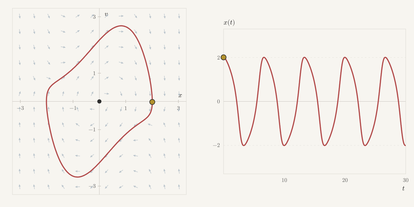
This system has a periodic solution. In the figure, a state goes around
a closed loop, swinging between about −2 and 2 and returning every
6.66 or so. The loop is not an ellipse, and its history 𝑥(𝑡) is not a
sine wave.
Figure 11.4 Left: the plane of 𝑥′=𝑣, 𝑣′=−𝑥+(1−𝑥2)𝑣. The red loop is a periodic
solution, with a state going around it in gold. Right: its history
𝑥(𝑡). Click the plane to release a state.
Every trajectory other than the equilibrium approaches this loop.
Release a state near the origin, and its small oscillation grows onto
the loop; release one far away, and its large oscillation shrinks onto
it. So this system has exactly one closed loop, and it attracts every
state except the origin. A linear flow has no closed loops or infinitely
many, and the size of its oscillation is set by where it starts. Here
the size is set by the equation, wherever the mass starts.
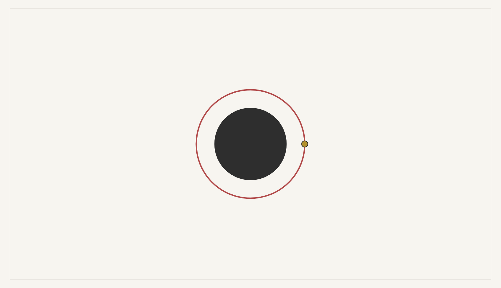
A closed orbit can also repel the states around it, and there is a famous
one in space. Light passing a black
hole bends toward it. Take a flat slice through the black hole, with its
center at the origin of the (𝑥,𝑦)-plane, and measure in units where
the black hole has radius 2. Describe a point on a light ray by its
distance 𝑟=√𝑥2+𝑦2 from the center and its angle 𝜃 around
it. The calculation that describes the ray comes from Einstein's theory
of gravity, but in the end it reduces to a differential equation for a
single variable, 𝑢=1/𝑟, as a function of the angle 𝜃:
𝑢″=−𝑢+3𝑢2.
This equation has a constant solution 𝑢=13: a circle of
radius 3, on which light orbits the black hole. This circle is called
the photon sphere.
Figure 11.5 Light near a black hole (the filled disk). The red circle is the photon
sphere, with light going around it in gold. Press and drag to aim a ray,
and release to fire it. The nudge button fires two rays from just inside
and just outside the photon sphere.
Light that starts near the photon sphere does not stay near it. Press
nudge in the figure: two rays start a millionth inside and a millionth
outside the photon sphere. They circle together nearly twice, then one
falls in and the other escapes. Van der Pol's loop pulls nearby
states onto it; this one pushes them away. Light coming in from far away
bends around the black hole, and the closer its path comes to the photon
sphere, the longer it circles before leaving.
The third property on our list, that every loop takes the same time,
fails too. In chapter 4 we followed the hare--lynx model
𝐻′=𝐻(1−𝐿),𝐿′=𝛾𝐿(𝐻−1),
and its trajectory appeared to make a closed loop around the equilibrium
(1,1). Take 𝛾=1. Every other state in the quadrant appears to lie
on such a loop, one through each state, like the circles of the spring
𝑥″=−𝑥. (We are still trusting the computation that the loops close.)
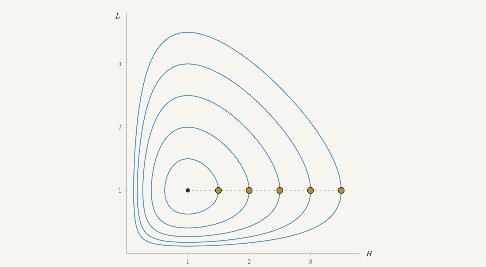
But the loops don't all take the same time to go around.
Figure 11.6 Closed loops of 𝐻′=𝐻(1−𝐿), 𝐿′=𝐿(𝐻−1), with one dot on each loop. The
dots start lined up on the dashed segment. Click to line them up again.
The dots start together and drift apart. The loop through (1.5,1)
takes about 6.38 to go around, and the loop through (3.5,1) takes
about 7.65: the bigger the swings in the populations, the longer a
cycle takes. In a linear center, the dots would stay lined up forever.
11.3Changing Parameters
A linear system 𝑋′=𝐴𝑋 in the plane is determined by the four entries of
𝐴, but its type depends on only two numbers, the trace and the
determinant. In section 8.4 we drew every possibility in one
picture, the trace–determinant plane. Moving the point
(tr𝐴,det𝐴) around can change the flow drastically: a
sink becomes a spiral sink, then a center, then a spiral source. But the
list of possible flows is short and fixed. There is exactly one
equilibrium, except on the horizontal axis, where a whole line of them
appears at once. Closed loops appear only on the half-line where the trace
is zero and the determinant is positive, and there every state lies on
one. Step off that half-line in any direction and all the loops disappear
together.
Let's see what two parameters can do in a nonlinear system. Start from the
hare--lynx model of chapter 4 with 𝛾=1, written with 𝑥 for the
prey and 𝑦 for the predators: 𝑥′=𝑥−𝑥𝑦, 𝑦′=−𝑦+𝑥𝑦. Now add three
effects:
The prey limit their own growth, as in logistic growth, through a term
−0.01𝑥2.
Each predator eats prey at a rate that levels off when prey are
plentiful, since a predator can only eat so fast. So 𝑥𝑦 becomes
𝑥𝑦/(1+𝛼𝑥).
The predators compete with each other, through a term −𝛿𝑦2.
The result is called Bazykin's model:
𝑥′=𝑥−𝑥𝑦1+𝛼𝑥−0.01𝑥2,𝑦′=−𝑦+𝑥𝑦1+𝛼𝑥−𝛿𝑦2.
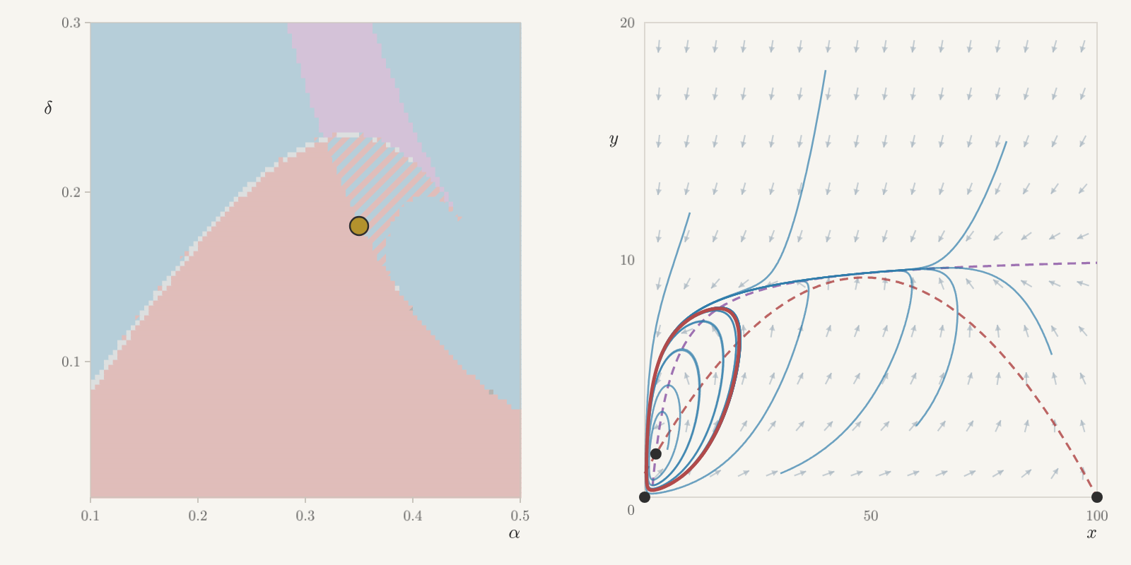
Each pair of numbers 𝛼, 𝛿 gives a different system, so the
pairs (𝛼,𝛿) form a plane of their own, just like the
trace–determinant plane.
Figure 11.7 Left: the plane of parameters (𝛼,𝛿) for Bazykin's model,
colored by what the populations end up doing. It is blue where every state
settles to one equilibrium, red where the populations cycle, violet where
they settle to one of two equilibria, and striped where some starting
populations cycle and others settle. Drag the gold point. Right:
trajectories for that choice of 𝛼 and 𝛿, with attracting
loops in red and the dashed curves where 𝑥′=0 and 𝑦′=0. Click to
release a state, and use the slider to zoom in on small populations.
The colors come from computing trajectories from many starting populations
at each point of a grid, so they are numerical evidence, not exact
boundaries. Start in the red region. The populations go around a single
closed loop, which attracts every state with both species present except
the equilibrium inside it, just like Van der Pol's loop. Here that happens
for a whole region of parameters, while a linear system has loops only
along one half-line. Drag up into the blue region and the loop is gone:
the populations settle to an equilibrium. In the violet region there are
three equilibria with both species present, and the populations settle to
one of two of them, depending on where they start. In the striped region,
a closed loop and an equilibrium attract at the same time: some starting
populations cycle forever, while others settle down. None of these can
happen in a linear system.
11.4Nearby States Drift Apart
In a linear system 𝑋′=𝐴𝑋, take two solutions 𝑋(𝑡)=𝑒𝑡𝐴𝑋0 and
𝑌(𝑡)=𝑒𝑡𝐴𝑌0. The gap between them is
𝑋(𝑡)−𝑌(𝑡)=𝑒𝑡𝐴(𝑋0−𝑌0),
which is just the solution starting from the initial gap 𝑋0−𝑌0. So
the gap does whatever every solution does. In a sink, it shrinks to
zero. In a center, it goes around a loop and never gets much bigger than
it started. The gap can only become large if solutions themselves grow
large, running off to infinity. So when solutions stay in a bounded
region, two states that start close together stay close together
forever.
In 1963 the meteorologist Edward Lorenz studied a simplified model of
convection in the atmosphere, with three unknowns:
𝑥′=10(𝑦−𝑥),𝑦′=𝑥(28−𝑧)−𝑦,𝑧′=𝑥𝑦−83𝑧.
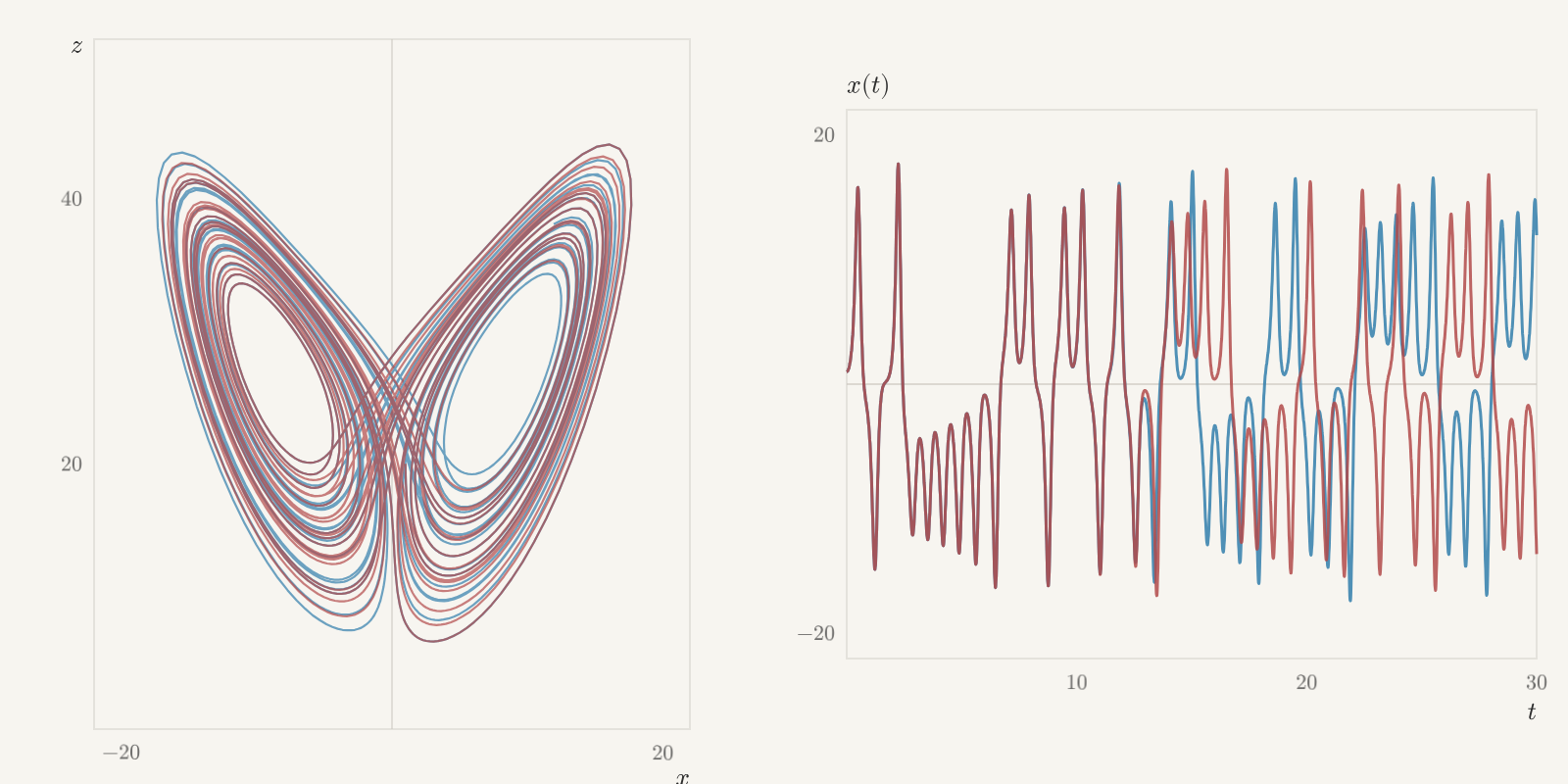
Its solutions stay in a bounded region of space, winding around two
lobes.
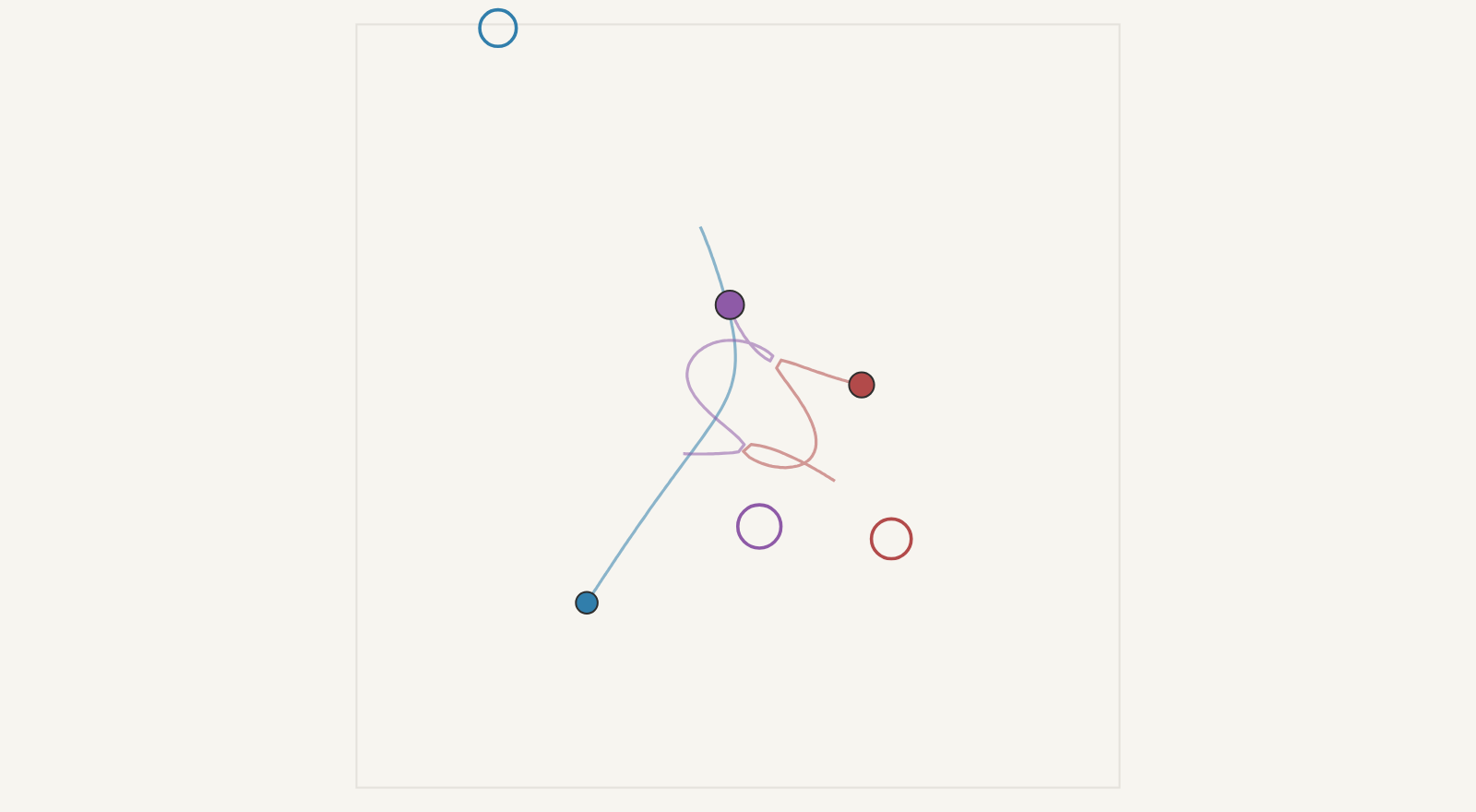
Figure 11.8 Two solutions of the Lorenz system, from (1,1,20) in blue and from
(1.00001,1,20) in red. Left: both trajectories seen from the side, in
the (𝑥,𝑧)-plane. Right: both histories 𝑥(𝑡). Click to watch again
from the start.
The two states start 0.00001 apart, and for a while they follow the
same path: their histories agree until about 𝑡=12. Then they come
apart and do completely different things, while both stay in the same
bounded region. Lorenz concluded that detailed weather forecasts far
into the future are impossible.
The same thing happens with gravity. Release three stars of masses 3,
4, and 5 from rest at the corners of a right triangle with sides
3, 4, and 5. Each star accelerates toward the other two by Newton's
law of gravitation: in units where the gravitational constant is 1,
star 𝑖 at position 𝑋𝑖 moves by
𝑋″𝑖=∑𝑗≠𝑖𝑚𝑗(𝑋𝑗−𝑋𝑖)|𝑋𝑗−𝑋𝑖|3.
Figure 11.9 Three stars of masses 3, 4, and 5, released from rest. The filled
dots are one run. The rings are a second run, with one star moved 0.001
at the start. Click to watch again from the start.
The rings sit on the dots until about 𝑡=40. After that, the two runs
have nothing to do with each other. In both systems, a change too small
to see at the start eventually changes everything.