In the last chapter, we computed the flow of every real 2×2
matrix. Choosing suitable coordinates revealed diagonal motion, rotation
with scaling, or shear with scaling. We now want to understand constant
linear systems with any number of unknowns:
𝑋′=𝐴𝑋,𝑋∈ℝ𝑛.
The matrix exponential already gives the solution, 𝑋(𝑡)=𝑒𝑡𝐴𝑋0.
Our task is to find coordinates that let us compute this flow and read
its motion. In a larger space, several different motions can occur at
once: one component of a state might grow along a line while another
rotates in a plane. We will begin with eigenvectors, where each component
evolves along its own line.
9.1Diagonalization
Let 𝑣 be a real eigenvector of 𝐴, with eigenvalue 𝜆. Since
𝐴𝑣=𝜆𝑣, we have 𝐴𝑘𝑣=𝜆𝑘𝑣 for every nonnegative integer
𝑘. Applying the exponential series to 𝑣 therefore gives
𝑒𝑡𝐴𝑣=∞∑𝑘=0𝑡𝑘𝐴𝑘𝑣𝑘!=∞∑𝑘=0(𝜆𝑡)𝑘𝑘!𝑣=𝑒𝜆𝑡𝑣.
The matrix exponential acts on an eigenvector by ordinary exponential
scaling. A state starting at 𝑐0𝑣 moves as 𝑐0𝑒𝜆𝑡𝑣, staying
on the same line. Thus eigenvectors identify invariant lines in
ℝ𝑛, just as they did in the plane.
If 𝐴 has a basis of real eigenvectors 𝑣1,…,𝑣𝑛, we already
know how to diagonalize it. With
𝑃=(𝑣1⋯𝑣𝑛),𝐷=diag(𝜆1,…,𝜆𝑛).
where 𝐴𝑣𝑗=𝜆𝑗𝑣𝑗, we have 𝐴=𝑃𝐷𝑃−1. Applying
theorem 8.1 from Chapter 8 gives
𝑒𝑡𝐴=𝑃𝑒𝑡𝐷𝑃−1=𝑃diag(𝑒𝜆1𝑡,…,𝑒𝜆𝑛𝑡)𝑃−1.
Multiplying by 𝑋0 gives the solution from any initial state. In
eigenvector coordinates, each component evolves by its own exponential;
in the original coordinates, each unknown is a linear combination of
those exponentials. The same diagonalization formula we used in the
plane solves every constant system that is diagonalizable over the reals,
in any dimension.
Example 9.1 (Four exponential components). Consider 𝑋′=𝐴𝑋, where
𝐴=⎛⎜
⎜
⎜
⎜
⎜
⎜
⎜⎝0120100220010210⎞⎟
⎟
⎟
⎟
⎟
⎟
⎟⎠.
The eigenvalues are 3,1,−1,−3. A corresponding matrix of eigenvectors
is
With these supplied, we can write the flow immediately:
𝑒𝑡𝐴=𝑃diag(𝑒3𝑡,𝑒𝑡,𝑒−𝑡,𝑒−3𝑡)𝑃−1.
Let's solve from 𝑋0=(1,0,0,0). We apply the factors in
𝑃𝑒𝑡𝐷𝑃−1𝑋0 from right to left. First multiply by 𝑃−1 to
find the initial state's eigenvector coordinates:
Now apply 𝑃𝑒𝑡𝐷 to this vector. The diagonal matrix 𝑒𝑡𝐷
multiplies each coordinate by its exponential, and 𝑃 converts the
result back to the original coordinates:
The state combines motion along four fixed eigendirections: two
components grow and two decay. Each original unknown mixes these
components, as the four entries of the solution show.
9.2Invariant Planes
What happens when the real eigenvectors do not form a basis? In two
dimensions, we encountered matrices with no real eigenvectors at all.
Their motion became rotation with scaling after a change of coordinates.
In higher dimensions, that same motion can occur on a plane inside the
larger state space.
Chapter 8 already tells us what rotation with scaling looks like in
suitable coordinates:
𝑅=(𝑎𝜔−𝜔𝑎),𝜔>0.
If we can find a plane on which 𝐴 has this matrix, we already know its
flow.
We want the characteristic polynomial to tell us which motions to look
for. A linear factor 𝑟−𝜆 gives an exponential rate 𝜆,
and we find its invariant line by solving (𝐴−𝜆𝐼)𝑣=0.
For a rotation plane, we need two numbers: a scaling rate 𝑎 and an
angular frequency 𝜔. These appear together in the characteristic
polynomial of 𝑅:
(𝑟−𝑎)2+𝜔2.
So we look for quadratic factors of the characteristic polynomial of 𝐴
that have no real roots. Completing the square identifies 𝑎 and
𝜔. Our next task is to find a plane carrying that motion.
Now we can reuse the basis construction from Chapter 8. Set 𝐵=𝐴−𝑎𝐼.
We want two independent vectors satisfying
𝐵𝑣=−𝜔𝑤,𝐵𝑤=𝜔𝑣.
The first equation tells us to choose
𝑤=−1𝜔𝐵𝑣.
The second will then hold precisely when
𝐵2𝑣=−𝜔2𝑣.
Here is what changes in higher dimensions. In Chapter 8, we proved
𝐵2=−𝜔2𝐼 on the whole space, so we could start with any nonzero
vector. Here we must find a vector on which that identity holds. We do
this by solving the homogeneous linear system
((𝐴−𝑎𝐼)2+𝜔2𝐼)𝑣=0,
For any nonzero solution, set 𝑤=−(𝐴−𝑎𝐼)𝑣/𝜔. The same check as
in Chapter 8 gives
𝐵𝑤=−1𝜔𝐵2𝑣=𝜔𝑣.
These vectors are independent. Otherwise 𝐵𝑣=𝑐𝑣 for some real number
𝑐, giving 𝐵2𝑣=𝑐2𝑣. But our equation says 𝐵2𝑣=−𝜔2𝑣, which
would require 𝑐2=−𝜔2.
Thus 𝑣,𝑤 span an invariant plane on which 𝐴 has matrix 𝑅. Chapter 8
supplies its motion: rotation at angular speed 𝜔, with scaling by
𝑒𝑎𝑡, in these coordinates.
We now have two related calculations:
Characteristic factor
Equation for 𝑣≠0
Invariant subspace
𝑟−𝜆
(𝐴−𝜆𝐼)𝑣=0
Line spanned by 𝑣
(𝑟−𝑎)2+𝜔2, 𝜔>0
((𝐴−𝑎𝐼)2+𝜔2𝐼)𝑣=0
Plane spanned by 𝑣,𝑤
The line carries the motion 𝑒𝜆𝑡𝑣. For the plane, set
𝑤=−(𝐴−𝑎𝐼)𝑣/𝜔; the motion is rotation with scaling.
9.2.1A Line and a Plane in Three Dimensions
Let's use both rows on a matrix we encountered in Chapter 7:
This matrix is not diagonal, but it contains a 1×1 matrix and a
2×2 matrix, with zeros between them. Our coordinates separate the
invariant line from the invariant plane.
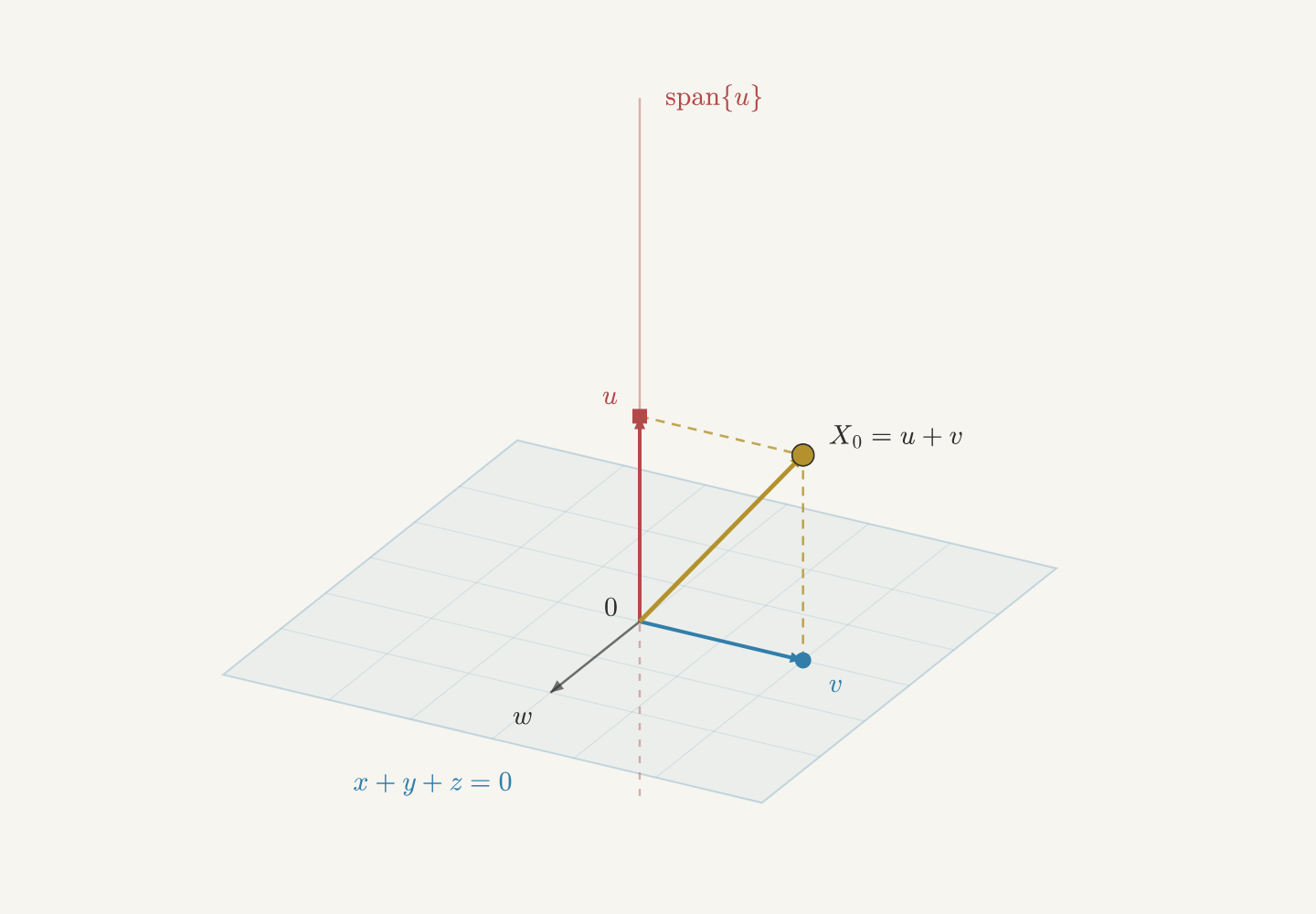
Figure 9.1 The state 𝑋0=(2,0,1)=𝑢+𝑣 splits into a component on the invariant
line and a component in the invariant plane. The dashed segments complete
their parallelogram. The vector 𝑤 supplies the other direction in the
plane. Rotate the view to see how these pieces sit in three dimensions.
The line and plane happen to be perpendicular for this matrix; an
invariant decomposition need not have that property.
Example 9.2 (Three lines and two planes). The same procedure works when several invariant lines and planes occur
together. Consider 𝑋′=𝐴𝑋 with
All seven coordinates are coupled. We will report the linear algebra
calculations and use their results to find coordinates built from three
invariant lines and two invariant planes.
Computing and factoring the characteristic polynomial gives
det(𝑟𝐼−𝐴)=(𝑟+1)(𝑟−1)(𝑟−3)(𝑟2+1)((𝑟+1)2+4).
The three linear factors give eigenvalues −1,1,3. The two quadratic
factors tell us to look for a plane with 𝑎=0, 𝜔=1, and another
with 𝑎=−1, 𝜔=2. Writing 𝑒1,…,𝑒7 for the standard
coordinate vectors, the calculations give these choices:
We have found coordinates that separate each matrix into smaller
blocks. We already know how to exponentiate those individual blocks.
Now we need to understand how their exponentials fit together.
A block-diagonal matrix has square matrices along its diagonal and
zeros everywhere outside those blocks:
The blocks need not have the same size. If 𝐵1 is 2×2 and 𝐵2
is 3×3, for example, placing them along the diagonal gives a
5×5 matrix. Each 0 in the display represents a whole rectangle
of zero entries of the appropriate size. We write this arrangement
compactly as 𝐶=diag(𝐵1,…,𝐵𝑟). An ordinary diagonal
matrix is the case in which every block has size 1×1.
To compute 𝑒𝑡𝐶, we need the powers of 𝐶. Start with two blocks.
Ordinary row-by-column multiplication gives
𝐶2=(𝐵100𝐵2)(𝐵100𝐵2)=(𝐵2100𝐵22).
Why do the blocks stay separate? To compute an entry in the upper-left
block, the only nonzero contributions come from multiplying entries of
𝐵1 by entries of 𝐵1. They give exactly the corresponding entry of
𝐵21. The lower-right block works the same way. For an entry outside
these two blocks, every product contains a zero, so the entry remains
zero.
Multiplying once more gives 𝐵31 and 𝐵32 in the same positions.
The same reasoning works for any number of blocks and every power:
𝐶𝑘=diag(𝐵𝑘1,…,𝐵𝑘𝑟).
This includes 𝑘=0: the identity matrix has an identity block of the
appropriate size in each position. Now the exponential series can be
summed separately in each block.
Theorem 9.3 (Exponentiating a block-diagonal matrix). Let 𝐵1,…,𝐵𝑟 be square matrices, possibly of different sizes,
and let 𝐶=diag(𝐵1,…,𝐵𝑟). Then
Thus we can exponentiate each diagonal block separately and put the
answers back in the same positions. If a change of coordinates gives
𝐴=𝑃𝐶𝑃−1 with 𝐶 block diagonal, Chapter 8 supplies the final step:
𝑒𝑡𝐴=𝑃diag(𝑒𝑡𝐵1,…,𝑒𝑡𝐵𝑟)𝑃−1.
We can now finish our two examples. For the three-dimensional system,
exponentiating the scalar block and the planar block gives
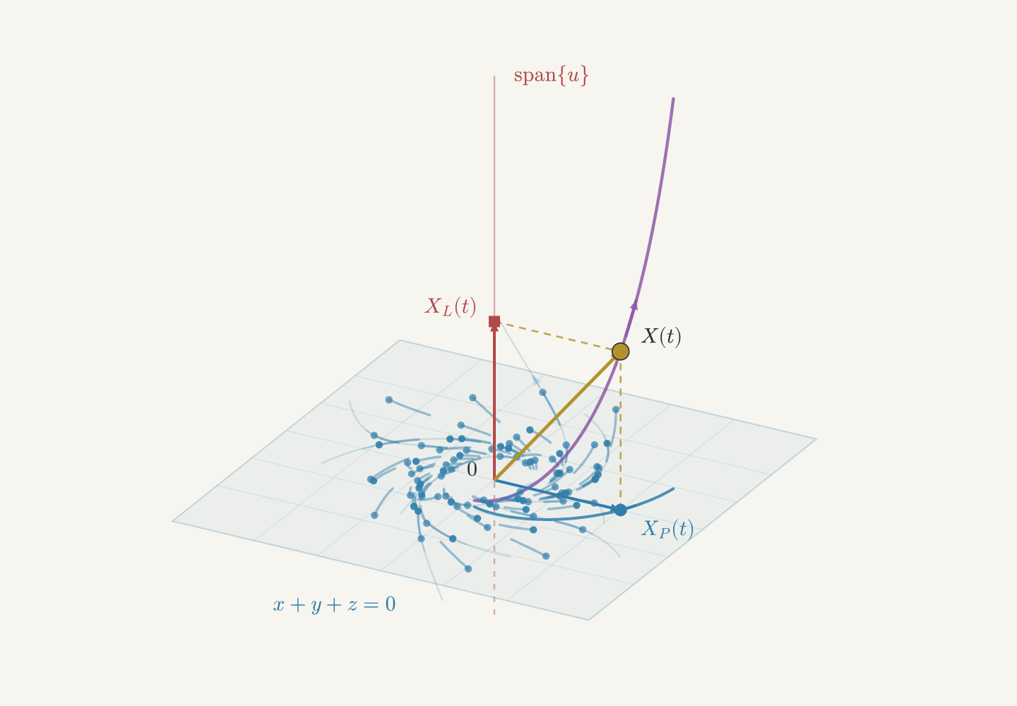
Figure 9.2 Watch the same parallelogram evolve. The red square 𝑋𝐿(𝑡) stays on
the invariant line, the blue point 𝑋𝑃(𝑡) stays in the invariant plane,
and their sum 𝑋(𝑡) follows the violet trajectory through space.
The surrounding blue points and their short trails show other solutions
spiraling outward, both within the plane and away from it. Use the time
slider to follow the motion, or rotate the view. The line component grows
faster than the plane component, so the displayed time interval is short;
playback restarts at the beginning of that interval.
The seven-dimensional example works the same way. Exponentiating its
three scalar blocks and two planar blocks gives
With the seven-dimensional matrix 𝑃 already calculated, the solution
is again
𝑋(𝑡)=𝑃𝑒𝑡𝐶𝑃−1𝑋0.
9.3Shear and Longer Chains
Our examples supplied a basis from invariant lines and rotation planes.
But Chapter 8 already showed that this can fail: shear has only one
eigenvector direction. In higher dimensions, the same coupling can
continue through more coordinates.
The characteristic polynomial is (𝑟−𝜆)3: the eigenvalue
𝜆 occurs three times. The diagonal matrix 𝜆𝐼 has
exactly the same characteristic polynomial, but every nonzero vector is
an eigenvector. For 𝐶, solving (𝐶−𝜆𝐼)𝑣=0 gives only the first
coordinate direction. The repeated eigenvalue alone does not tell us
whether we have independent eigendirections or a coupled chain.
Nevertheless, the exponential is easy to compute. Since 𝑁3=0, the
series stops:
The quadratic term comes from two successive couplings. After removing
the uniform exponential scaling, the equations are 𝑥′=𝑦, 𝑦′=𝑧,
𝑧′=0. A constant 𝑧 produces a linear term in 𝑦, which produces a
quadratic term in 𝑥.
What basis puts a matrix 𝐴 into this form? With 𝑃=(𝑣1𝑣2𝑣3),
the equation 𝐴𝑃=𝑃𝐶 says
(𝐴−𝜆𝐼)𝑣1=0,(𝐴−𝜆𝐼)𝑣2=𝑣1,(𝐴−𝜆𝐼)𝑣3=𝑣2.
These vectors form a chain: applying 𝐴−𝜆𝐼 sends each vector
to the preceding one, and sends the first to zero. Only the first is an
eigenvector. If we find a basis with these relations, the solution is
𝑋(𝑡)=𝑃𝑒𝑡𝐶𝑃−1𝑋0, using the exponential just computed.
A longer chain works the same way. For a chain of length 𝑚, the
matrix is
Here 𝑁 has ones immediately above the diagonal and zeros elsewhere,
so 𝑁𝑚=0. A matrix whose powers eventually vanish is called
nilpotent. The exponential series again terminates:
Thus a chain of length 𝑚 contributes 𝑒𝜆𝑡 times polynomials
of degree at most 𝑚−1. Its coordinates are coupled; the whole chain
forms one block to use in our block-diagonal solution formula.
Rotation blocks can be coupled in the same way. Take
𝑅=(𝑎𝜔−𝜔𝑎),𝜔>0,
and form the 4×4 matrix
𝐶=(𝑅𝐼0𝑅)=(𝑅00𝑅)+(0𝐼00),
where each 𝐼 is the 2×2 identity. Its characteristic polynomial
is
det(𝑟𝐼−𝐶)=((𝑟−𝑎)2+𝜔2)2.
Here the same quadratic factor occurs twice. Removing the off-diagonal
𝐼 would give diag(𝑅,𝑅), with the same characteristic
polynomial but two independent rotation planes. In 𝐶, the 𝐼 couples
them into a chain.
The two summands in our split of 𝐶 commute, and the second squares to
zero. We can therefore exponentiate them separately:
𝑒𝑡𝐶=(𝑒𝑡𝑅00𝑒𝑡𝑅)(𝐼𝑡𝐼0𝐼)=(𝑒𝑡𝑅𝑡𝑒𝑡𝑅0𝑒𝑡𝑅).
We already know 𝑒𝑡𝑅 from Chapter 8. The coupling adds a factor of
𝑡, so the entries now include 𝑡𝑒𝑎𝑡cos(𝜔𝑡) and
𝑡𝑒𝑎𝑡sin(𝜔𝑡).
Longer chains repeat the same block 𝑅 along the diagonal, with 𝐼
immediately above it. The same calculation puts 𝑒𝑡𝑅 on the
diagonal, 𝑡𝑒𝑡𝑅 immediately above it, then
𝑡22!𝑒𝑡𝑅, and so on. A chain of 𝑚 rotation blocks
therefore contributes polynomials of degree at most 𝑚−1 multiplying
𝑒𝑎𝑡cos(𝜔𝑡) and 𝑒𝑎𝑡sin(𝜔𝑡).
In both cases, a chain longer than one requires a repeated factor in the
characteristic polynomial. Repeated factors make these chains possible;
they do not force them. The extra powers of 𝑡 come from the coupling
within a chain.
9.4Real Jordan Form
Most real matrices can be put into a form like this:
The lines mark three diagonal blocks: the number 3, a 2×2
rotation block, and another 2×2 rotation block. Everything
outside those blocks is zero. This five-dimensional system separates
into one scalar equation and two independent planar systems. We know
how to solve all three.
Repeated eigenvalues can require a larger block. For example,
This matrix is still block diagonal, but now it has two blocks. The
first is a three-dimensional chain for the repeated eigenvalue 2;
its coordinates are coupled by the two ones above the diagonal. The
second is an independent rotation block. The whole chain is one
block, and we exponentiate it as a unit.
Here the ones in positions (1,3) and (2,4) couple the two coordinate
pairs. This is one four-dimensional chain block. If those two ones
were zero, we would instead have two independent 2×2 blocks.
These matrices are examples of real Jordan form. The theorem says
that every real matrix can be put into block-diagonal form using just
these kinds of blocks: numbers, rotation blocks, and chains.
Theorem 9.4 (Real Jordan form). Let 𝐴 be a real 𝑛×𝑛 matrix.
If no characteristic factor repeats, there is a real invertible
matrix 𝑃 such that 𝑃−1𝐴𝑃 is block diagonal with only real numbers
and 2×2 blocks of the form
𝑅=(𝑎𝜔−𝜔𝑎),𝑎∈ℝ,𝜔>0.
Each real linear factor supplies one eigenvector direction, and each
quadratic factor with no real roots supplies one invariant plane.
Together these give a basis of the whole space. If there are 𝑝 linear
factors and 𝑞 quadratic factors, then 𝑝+2𝑞=𝑛.
For every real matrix, there is still such a block-diagonal form if
we also allow the chains from the preceding section: copies of the same
real number linked by ones, or copies of the same rotation block linked
by 2×2 identity matrices. Chains may have any length. A chain
longer than one requires a repeated characteristic factor, but repeated
factors do not force longer chains.
We state the existence of these coordinates without proof; that is the
linear algebra result. We have already done the differential equations:
if the diagonal blocks are 𝐽1,…,𝐽𝑠, the solution is
𝑋(𝑡)=𝑃diag(𝑒𝑡𝐽1,…,𝑒𝑡𝐽𝑠)𝑃−1𝑋0,
and every exponential on the right is one we have computed.
9.5The Form of Every Solution
Real Jordan form tells us that our list of blocks is complete. So our
calculations also give a complete list of the kinds of functions that
can appear in a solution.
Block
Functions appearing in its solutions
A real eigenvalue 𝜆
𝑒𝜆𝑡
A rotation block
𝑒𝑎𝑡cos(𝜔𝑡), 𝑒𝑎𝑡sin(𝜔𝑡)
A real chain of length 𝑚
𝑡𝑘𝑒𝜆𝑡
A chain of 𝑚 rotation blocks
𝑡𝑘𝑒𝑎𝑡cos(𝜔𝑡), 𝑡𝑘𝑒𝑎𝑡sin(𝜔𝑡)
For rotation blocks, 𝑎 is the exponential scaling rate and 𝜔
is the frequency. In the chain rows, 0≤𝑘<𝑚: the chain lengths
bound the powers of 𝑡 that can occur. A particular
initial condition may make some of their coefficients zero.
These are the functions we see in Jordan coordinates. Why do they also
describe the original unknowns? Write 𝐶=𝑃−1𝐴𝑃 and recall that
𝑋(𝑡)=𝑃𝑒𝑡𝐶𝑃−1𝑋0.
The vector 𝑃−1𝑋0 is constant, so multiplying 𝑒𝑡𝐶 by it takes
linear combinations of the entries of 𝑒𝑡𝐶. Multiplying by 𝑃
takes further linear combinations. Neither step introduces any new
kind of time dependence.
Thus, for every real constant matrix 𝐴, each component of every
solution of 𝑋′=𝐴𝑋 is a finite linear combination of functions of the
forms
𝑡𝑘𝑒𝜆𝑡,𝑡𝑘𝑒𝑎𝑡cos(𝜔𝑡),𝑡𝑘𝑒𝑎𝑡sin(𝜔𝑡).
The matrix determines which rates, frequencies, and polynomial degrees
are available; the initial condition determines their coefficients.
These are all the functions we need, no matter how many unknowns the
system has.
Problems
1A flow in three dimensions
Consider the system
𝑥′=2𝑦−3𝑧,𝑦′=3𝑥−𝑦−3𝑧,𝑧′=−2𝑥+2𝑦−𝑧.
(a)
Write the matrix of this system, and find and factor its characteristic
polynomial. Then find an eigenvector for each eigenvalue.
(b)
Find the solution with 𝑥(0)=1, 𝑦(0)=0, 𝑧(0)=0.
(c)
Describe what happens to solutions as 𝑡→∞. Which initial states
give solutions that approach the origin? What happens to every other
solution, and how can you tell from the initial state which way it
heads?
2A flow with an invariant plane
Consider the system
𝑥′=2𝑦+2𝑧,𝑦′=𝑥−𝑦−2𝑧,𝑧′=−2𝑥−𝑦.
Let 𝐴 be the matrix of this system. In Chapter 9, a quadratic factor
with no real roots led us to an invariant plane. Here is the procedure.
First complete the square to
write the factor as (𝑟−𝑎)2+𝜔2 with 𝜔>0. Then find a
nonzero vector 𝑣 solving
((𝐴−𝑎𝐼)2+𝜔2𝐼)𝑣=0,
and set
𝑤=−1𝜔(𝐴−𝑎𝐼)𝑣.
Then 𝐴𝑣=𝑎𝑣−𝜔𝑤 and 𝐴𝑤=𝜔𝑣+𝑎𝑤. So 𝑣 and 𝑤 span a plane
that the flow never leaves, and in the basis 𝑣,𝑤 the matrix of 𝐴 on
this plane is
(𝑎𝜔−𝜔𝑎),withflow𝑒𝑎𝑡(cos𝜔𝑡sin𝜔𝑡−sin𝜔𝑡cos𝜔𝑡).
On this plane, states rotate at angular speed 𝜔 while scaling by
𝑒𝑎𝑡.
(a)
Write the matrix of this system, and find and factor its characteristic
polynomial. What motion does each factor describe? For the linear
factor, give the exponential rate along its line. For the quadratic
factor, give the scaling rate and the time for one full turn in its
plane.
(b)
Find an eigenvector 𝑢 for the linear factor. Then use the procedure above
to find vectors 𝑣 and 𝑤 spanning the invariant plane.
(c)
Find the solution with 𝑥(0)=2, 𝑦(0)=−1, 𝑧(0)=0.
(d)
Describe what happens as 𝑡→∞ to solutions starting on the
invariant line, solutions starting in the invariant plane, and solutions
starting anywhere else.
3Splitting a matrix into commuting pieces
In each part, write the matrix as a sum of two pieces that commute, and
use this to compute its exponential.
where 𝐼 is the 2×2 identity and 0 is the 2×2 zero
matrix.
4Reading the motion from the characteristic polynomial
A 6×6 matrix 𝐴 has characteristic polynomial
(𝑟+3)(𝑟−1)(𝑟2+4)(𝑟2+2𝑟+5).
We do not need the matrix itself to understand the motion of 𝑋′=𝐴𝑋.
(a)
Make a table with one row for each factor. In each row, record whether
the factor gives an invariant line or an invariant plane, whether the
motion there grows, decays, or neither, and the period of any
oscillation.
(b)
Describe what happens as 𝑡→∞ to the solution starting from each
of these states:
a state on the invariant line from 𝑟+3;
a state in the invariant plane from 𝑟2+4;
a state with components only in the two invariant planes;
a state with a nonzero component on the invariant line from 𝑟−1.
5The repressilator
Every cell carries instructions for building proteins in its genes. To
make a protein, the cell copies a gene into a molecule called mRNA, then
builds the protein from that copy. Some proteins are repressors: a
repressor binds to the DNA at the start of another gene and blocks that
gene from being copied. The more repressor there is, the less of the
other protein gets made. Proteins don't last forever, either. The cell
breaks them down, and they are diluted as the cell grows and divides.
In 2000, Michael Elowitz and Stanislas Leibler used these ingredients to
build a biological clock from scratch in the bacterium E. coli. They
chose three repressor genes that occur in no natural clock and arranged
them in a ring:
the protein LacI represses the gene for TetR;
the protein TetR represses the gene for CI;
the protein CI represses the gene for LacI.
They called the circuit the repressilator. To watch it, they added a
gene for a green fluorescent protein that TetR also represses, so a cell
glows when its TetR level is low. Under a microscope, individual cells
blinked on and off, with a period of around 150 minutes. That is about
three times as long as it takes the cells to divide.
Why would this ring oscillate? Suppose a cell has a little extra LacI.
Extra LacI shuts down TetR production, so TetR falls. With less TetR, the
gene for CI is released, so CI rises. Extra CI shuts down LacI
production, so LacI falls. The original excess of LacI has come back
around the ring as a shortage of LacI. Each step takes time, because
proteins are built and removed gradually, so the levels keep
overshooting. Whether these swings die away or grow depends on how
strongly each repressor acts. That is what we can decide with linear
algebra.
Here is a simplified model, which tracks only the proteins. In a steady
state, all three proteins sit at the same level, with production exactly
balancing removal. Let 𝑥, 𝑦, and 𝑧 be the deviations of LacI, TetR,
and CI from that steady level. We measure time in units of a protein's
lifetime, so each protein is removed at rate equal to its own deviation.
Each production rate is a decreasing function of the repressor upstream
of it. For small deviations, we replace that curve by its tangent line,
whose slope we write as −𝐾. This gives
𝑥′=−𝑥−𝐾𝑧,𝑦′=−𝑦−𝐾𝑥,𝑧′=−𝑧−𝐾𝑦.
For example, the term −𝐾𝑥 in the equation for 𝑦′ says that extra
LacI (𝑥>0) lowers TetR production. The constant 𝐾>0 measures how
sharply production responds to its repressor.
(a)
Write the matrix of this system, and find and factor its characteristic
polynomial. Don't multiply out (𝑟+1)3. Instead, write 𝑠=𝑟+1 and use
the identity
𝑠3+𝐾3=(𝑠+𝐾)(𝑠2−𝐾𝑠+𝐾2),
which you can check by multiplying out the right side. Then complete the
square in the quadratic factor.
(b)
The quadratic factor describes oscillation in an invariant plane. Find
its frequency and its scaling rate in terms of 𝐾.
(c)
If the oscillations in the invariant plane die out, the protein levels
settle back to their steady state, and the clock stops ticking. For the
circuit to work as a clock, the oscillations must grow, so that they
become large enough to notice and measure. For which values of 𝐾 does
this happen?
6Possible or impossible?
Each part names a function and the size of a constant system 𝑋′=𝐴𝑋.
Decide whether the function can appear as a component of some solution of a
system of that size. If it can, describe blocks of a real Jordan form that
would produce it. If it cannot, explain why not.
(a)
𝑡𝑒𝑡cos𝑡, for a 3×3 system.
(b)
𝑡2𝑒𝑡, for a 2×2 system.
(c)
𝑒𝑡cos𝑡+𝑒2𝑡cos3𝑡, for a 3×3 system. What about a 4×4
system?
(d)
𝑡𝑒−𝑡+𝑒2𝑡, for a 3×3 system.
(e)
𝑒𝑡+𝑒2𝑡+𝑒3𝑡+𝑒4𝑡, for a 3×3 system.
7Same polynomial, different flows
Consider the two systems
𝑥′=2𝑥,𝑦′=2𝑦,𝑧′=𝑥−𝑧and𝑥′=2𝑥+𝑦,𝑦′=2𝑦,𝑧′=𝑥−𝑧.
They differ in a single term.
(a)
Show that both matrices have characteristic polynomial (𝑟−2)2(𝑟+1).
(b)
For each system, find all eigenvectors for the eigenvalue 2 and for the
eigenvalue −1. Which system has an eigenvector basis?
(c)
For the second system, let 𝐴 be its matrix and 𝑣1 its eigenvector for
the eigenvalue 2. Find a vector 𝑣2 with (𝐴−2𝐼)𝑣2=𝑣1. Write down the
real Jordan form of each matrix.
(d)
Solve both systems from (𝑥,𝑦,𝑧)=(0,1,0). Which function appears in one
solution but not the other, and where does it come from?
8A third-order equation
Consider the equation 𝑥‴=𝑥.
(a)
Write it as a system 𝑋′=𝐴𝑋 with state 𝑋=(𝑥,𝑥′,𝑥″). Find and factor the
characteristic polynomial of 𝐴.
(b)
Find the invariant line and the invariant plane, with the scaling rate and
frequency of the motion in the plane.
(c)
Which functions can appear in a solution 𝑥(𝑡)? Which initial data
(𝑥(0),𝑥′(0),𝑥″(0)) give solutions that decay to zero? What happens to
every other solution?
(d)
Compare 𝐴 with the matrix in A Line and a Plane in Three Dimensions. How
are the two matrices related, and why do they share the same invariant line
and plane?
9Two independent pieces
Consider the system
𝑥′=3𝑦,𝑦′=−3𝑥,𝑧′=−𝑧+𝑤,𝑤′=−𝑤.
(a)
Write the matrix of this system and explain why it is block diagonal. What
is each block?
(b)
Exponentiate each block and assemble 𝑒𝑡𝐴.
(c)
Find the solution from (𝑥,𝑦,𝑧,𝑤)=(1,0,0,1).
(d)
Describe the solution as 𝑡→∞. Which initial states give periodic
solutions?
10A cascade, solved two ways
Consider the system
𝑥′=𝑥+𝑦,𝑦′=2𝑦+𝑧,𝑧′=3𝑧,
with (𝑥,𝑦,𝑧)=(0,0,1) at 𝑡=0.
(a)
Solve the third equation, substitute into the second and solve it, then do
the same for the first. Use the methods of Chapter 2.
(b)
Explain why the eigenvalues of this matrix can be read from its diagonal.
Find an eigenvector for each eigenvalue.
(c)
Write (0,0,1) in the eigenvector basis and write the solution as a
combination of exponential motions. Check that it agrees with part (a).
11Finding a chain
Let 𝐴 be the matrix of the system
𝑥′=−2𝑥+𝑦,𝑦′=−𝑦+𝑧,𝑧′=𝑥−𝑦.
(a)
Show that the characteristic polynomial is (𝑟+1)3 and that there is only
one independent eigenvector.
(b)
Let 𝑁=𝐴+𝐼. Compute 𝑁2 and 𝑁3. Use them to find 𝑒𝑡𝐴=𝑒−𝑡𝑒𝑡𝑁.
(c)
Start from 𝑣3=(0,0,1) and set 𝑣2=𝑁𝑣3 and 𝑣1=𝑁𝑣2. Check that
𝑁𝑣1=0. Explain why, in the basis 𝑣1,𝑣2,𝑣3, the matrix of 𝐴 is a
chain of length 3.
(d)
Find the solution from (0,0,1). Which powers of 𝑡 appear?